5.3 Accidents of birth: Another lens for studying inequality
Much inequality in the world today can be traced to differences among people over which they have virtually no control, such as their race, sex, nation, or parents.
We call these differences accidents of birth because people have no control over them at birth.
Categorical inequality and institutions
Race and persistent inequality in the United States
If you are interested in learning more about race and the persistence of racial inequality in the United States, consider reading CORE Econ’s Insight, “Persistent Racial Inequality in the United States.”
- group or categorical inequality
- Inequality between particular social groups (identified, for instance, by a category such as race, nation, caste, gender, or religion). Also known as group inequality.
Inequalities based on one’s ethnic identity or caste are examples of categorical inequality, also known as group inequality. Categorical inequality refers to economic differences among people who are treated as being in different social categories as defined by more powerful social classes. “African American” or “Black” is a category, as are “white,” “Hispanic,” “Asian American,” and “Native American” in the United States. For the most part, categorical inequalities are based on accidents of birth, because people are born into membership in one or more of the categories, and switching categories is typically difficult and maybe even impossible.
- correspondence study
- A type of experiment in which experimenters send out fictitious applications submitted online or via the mail. The experimenters randomly vary the specific characteristics they are interested in studying.
How can we measure such group inequality? In one approach, called a correspondence study, experimenters send out to prospective employers fake résumés of qualified candidates, who differ only in their category or group membership as revealed in the résumé, for example by names that are typically male or female or (in the US) African American or European American (the terms used in the original research). Before sending these résumés, the experimenters randomly vary specific characteristics, such as race, gender, or employment history. In 2020, economists Patrick Kline, Evan Rose, and Christopher Walters did just such an experiment with employers across the US, sending the résumés of over 83,000 fictitious applicants to 108 of the biggest US employers.
In their study, Kline et al. differentiated people using distinctive names. They used a database of distinctive first names combined with last names based on the 2010 census. For example, a previous study using a similar method used the names Lakisha and Jamal as distinctively Black first names whereas Emily and Greg are distinctively white first names. Data Extension 10.5a explores other results of correspondence studies in greater detail, with particular applications to the labor market.
Job applicants with distinctively white names were 10% more likely to be contacted by employers than applicants with distinctively Black names.
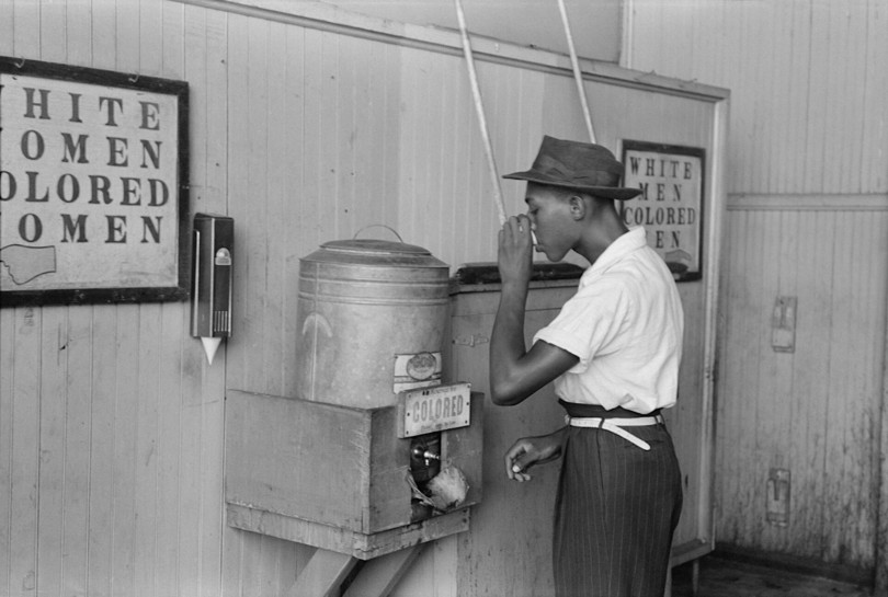
A photograph titled “Negro drinking at ‘Colored’ water cooler in streetcar terminal, Oklahoma City, Oklahoma,” by Russell Lee (1903–1986). This photo captures the ways in which Jim Crow laws, which enforced racial segregation in the United States, affected the everyday lives of Black Americans, who were required to use different services than white Americans used.
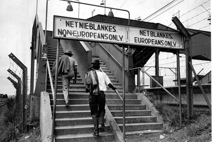
A segregated bridge at Pretoria railway station, South Africa, 1960s, photograph by Ernest Cole (1940–1990). The photo shows how South Africa’s apartheid system of formalized racial segregation, in which white South Africans had voting rights and non-white South Africans did not, meant segregating people even when they were crossing railway bridges to prevent any intermingling of the races.
Inequalities based on categorical inequalities such as race may be perpetuated by institutions and social norms, as in the following examples:
- Formalized discrimination. The Jim Crow regime was a set of laws (and informal social norms) in the United States to formalize racial discrimination. The laws lasted roughly until the 1964 Civil Rights Act, which prohibits discrimination based on race, color, religion, sex, and national origin.
- Colonists and Indigenous people. In Australia, the United States, parts of Africa, and much of Latin America, extreme economic and social inequalities exist between descendants of European colonists and the descendants of those who lived in the territory prior to the colonists’ arrival, called Indigenous peoples. The laws in many of these countries—for example, the formalized racial policies in South Africa, collectively termed apartheid—privileged the colonists and other groups over Indigenous peoples.
- Caste. Vast disparities in life chances in India follow from long-established hereditary and hierarchical boundaries determined by caste, a form of social stratification based on historical social norms and on the legal reinforcement of these rules during British colonial rule. Caste is a social status that ranges from high-status Brahmins to low-status Dalits (once called “untouchables”) and is reinforced through institutions and social norms forbidding marriage across caste.
Everyday Economics 5.4
One important form of categorical inequality is gender inequality. We explore the consequences of gender inequality in the labor market in Chapter 10. In what ways does gender inequality alter the goals people are able to pursue and the constraints they face? What institutions or social norms relate to the prevalence of gender inequality? Which factors reduce gender inequality?
Categorical inequalities come to exist for a variety of reasons and may then persist through formal institutions, such as the segregationist laws in South Africa and the United States described above, or through informal institutions, such as the social norms around marriage across caste in India. Laws may be revoked or passed through collective action and democratic processes, such as the Civil Rights Movement in the United States, which culminated in the Civil Rights Act, or the anti-apartheid movement in South Africa and internationally that democratically overturned the South African government in 1994. Informal institutions may change as a result of evolving social norms. For example, parents may teach their children different values, and the institutions that children learn to uphold through schooling or in their neighborhood or social connections may change due to the behaviors of neighbors and friends.
Intergenerational inequality
A second source of inequality exists across generations: Children tend to inherit their economic status from their parents. You may be rich or poor because your parents were rich or poor. Meanwhile, others may inherit family businesses and social status without having to prove that they are the best person for the job.
Everyday Economics 5.5
Many genetic and biological factors play a role in intergenerational inequality. Consider, for example, perceived attractiveness. Perceived attractiveness has genetic, nutritional, and effort components. Nonetheless, the role of genetically inherited attributes from parents remains important. Using paired parent and child data, economists Daniel S. Hamermesh and Anwen Zhang showed a correlation between the perceived attractiveness of parents and that of their children in the United States and China. According to their research, when parents are more attractive, their children earn more income when they are adults. Why do you think this might be true? What other attributes do you think might have genetic or biological components that can affect intergenerational inequality in similar ways?
- intergenerational inequality
- The extent to which differences in parental generations are passed on to the next generation, as measured by the intergenerational elasticity or the intergenerational correlation. See also intergenerational mobility, intergenerational elasticity.
Intergenerational inequality occurs when the inheritance process results in similarity between the economic status of parents and their children: the children of rich people become rich, while the children of poor people stay poor. The transmission of inequality from parents to children can occur through three mechanisms:
- Children inherit the wealth of their parents, and the quality and quantity of their education tend to be similar.
- The children’s genetic makeup is similar to that of their parents, affecting physical characteristics (such as height) and performance on cognitive tests.
- Parents and children tend to share similar preferences, social norms, knowledge, skills, and social connections acquired outside formal schooling.
Researchers measure intergenerational inequality by ranking parents’ incomes and then looking at their adult children’s income. Children whose parents had a high income tend to have high incomes as adults, and children from low-income families tend to have low incomes as adults. But how strong is this tendency, and does it vary across countries? Figure 5.5 compares the answer for three countries—the United States, Denmark, and Australia—using administrative tax records that cover millions of parent–child pairs.
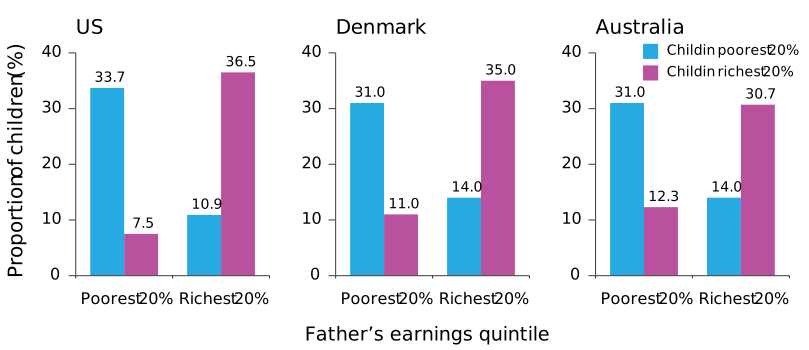
Figure 5.5 Intergenerational inequality in labor earnings: the United States, Denmark, and Australia. The percentage of adult children in the poorest 20% is shown in blue, and the percentage of children in the richest 20% is shown in pink. If outcomes were random, each bar would equal 20%.
Chetty, Raj, Nathaniel Hendren, Patrick Kline, and Emmanuel Saez. 2014. “Where is the Land of Opportunity: The Geography of Intergenerational Mobility in the United States”. Quarterly Journal of Economics 129 (4): 1553-1623.
Jesper Eriksen. 2018. Finding the Land of Opportunity Intergenerational Mobility in Denmark. Table II.
Nathan Deutscher, Bhaskar Mazumder. 2020. ‘Intergenerational mobility across Australia and the stability of regional estimates’. Labour Economics 66.
Axes to compare the father’s earning quintile and child’s earning quintile in the United States, Denmark, and Australia
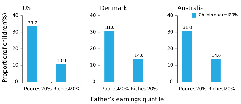
Father’s income quintiles and children who are in the poorest 20% in the United States, Denmark, and Australia
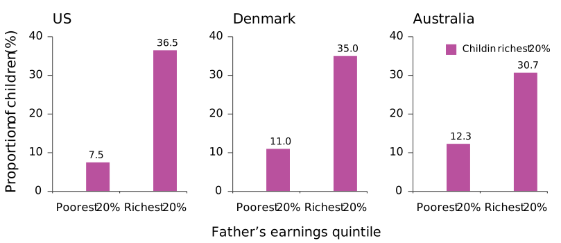
Father’s income quintiles and children who are in the richest 20% in the United States, Denmark, and Australia
Father’s income quintiles and children’s income quintiles in the United States, Denmark, and Australia
The horizontal axis in each panel groups children by their father’s income. The bars show what fraction of those children ended up in the poorest 20% (blue) or the richest 20% (pink) of their own generation. A benchmark to keep in mind: if family background had no effect on a child’s income, then each bar would equal 20%, because every child would have an equal chance of ending up in any quintile.
- Poor staying poor: In the United States, 33.7% of children born to fathers in the poorest 20% ended up in the poorest 20% of adults—nearly one and a half times the 20% that random chance would predict—and only 7.5% made it to the richest 20%. Denmark and Australia both show lower bottom-quintile “stickiness”: 31% of children born to the poorest 20% of fathers remained there in both countries. More strikingly, 11% of children born at the bottom in Denmark and 12.3% in Australia reached the richest 20% as adults—well above the US figure of 7.5%.
- Rich staying rich: In the United States, 36.5% of children born to the richest 20% of fathers stayed in the richest 20% as adults. In Denmark the figure is 35%, and in Australia it is notably lower at 30.7%. At the same time, 14% of the richest fathers’ children fell to the bottom quintile in both Denmark and Australia, compared with only 10.9% in the United States. Privilege is more persistent in the United States not only because disadvantage is stickier at the bottom, but also because advantage is stickier at the top.
- progressiveness of tax-and-transfer systems
- The progressiveness of a tax-and-transfer system describes the extent to which taxes and government transfers reduce inequality in disposable income by taking a larger share from people with higher incomes and/or directing more support to people with lower incomes.
Children of the rich tend to be richer than children of the poor partly because of the financial support that rich parents give their children, both during the parents’ lifetimes and at death in the form of inheritances. The data in Figure 5.5 are based on family income or its close equivalent, not inherited wealth alone, so the data also capture intergenerational advantages in schooling quality, parental connections, and social capital. These factors operate with different force across countries because of differences in public investment in early childhood and schooling, in the progressiveness of tax-and-transfer systems, and in the degree of wage inequality that separates the top from the bottom of the income distribution.
We can conclude that intergenerational inequality is substantial in all three countries, but it is notably higher in the United States. Denmark and Australia both achieve greater mobility from the bottom—the “American Dream” measure of bottom-to-top movement is roughly one and a half times higher in those countries than in the United States—and lower persistence of advantage at the top. None of the three countries comes close to the 20% random-chance benchmark, which would represent a completely level playing field.
Exercise 5.3 Estate and inheritance tax in the United States
- Explain how inherited wealth contributes to intergenerational inequality.
- The US federal estate tax is a tax on the net value of a deceased person’s estate before it is distributed to heirs. The estate is taxed only above a large exemption threshold, and the taxable amount is reduced by deductions (amounts subtracted before tax, such as bequests to a spouse or to charity) and exclusions (transfers that are not counted, such as gifts made during the person’s lifetime up to an annual limit).
- Briefly research and describe how the federal estate tax works. In your answer, identify the current exemption threshold and at least two deductions or exclusions that reduce the amount of an estate that is taxed.
- Evaluate how effective the estate tax is at redistributing wealth. In particular, explain how the high exemption threshold and the available deductions and exclusions affect how much wealth the tax actually redistributes, and therefore its effect on inequality.
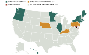
- As shown on the map in Exercise Figure 5.3 (i), some US states also levy additional estate or inheritance taxes. What are some possible reasons why many other states choose not to impose such taxes?
Exercise Figure 5.3 (i)
States with estate taxes, inheritance taxes, both kinds of taxes, or neither. These are state-level taxes levied in addition to the federal estate tax discussed in question 2 above: a few states impose their own estate or inheritance tax on top of the federal tax, while most do not. The interactive version also includes information about the rates of taxation and their cutoffs.
Tax Foundation, Bloomberg, and State Statutes.
Exercise 5.4 Understanding the correspondence study
In the correspondence study by Kline, Rose, and Walters (described in Section 5.3), in 2020 the researchers sent fictitious résumés to 108 of the largest US employers. Applicants with distinctively white names were 10% more likely to be contacted than applicants with distinctively Black names. Use the description of this study, together with Section 5.3, to answer the questions below.
- Using this study as an example, explain what a correspondence study is and why economists use this method rather than simply comparing the wages of Black workers and white workers.
- The study held constant factors such as education, work experience, and the quality of the résumé. Which methodological assumption does this reflect? Why is it important?
- Explain how the finding that white-named applicants were 10% more likely to be contacted constitutes evidence of categorical inequality. What kind of institution or social norm does this finding suggest is operating in these firms’ hiring practices?
Question 5.4
Which of the following is an example of categorical inequality?
- Differences in education level alone do not represent categorical inequality, which is based on social categories.
- This answer choice refers to individual differences in behavior, not inequality based on social categories.
- Categorical inequality refers to economic differences based on factors such as race, caste, or gender, which are outside an individual’s control.
- Categorical inequality is not about personal effort; it is about structural barriers experienced by identity groups.
Question 5.5
According to Figure 5.5, which of the following statements about intergenerational income mobility are correct? Choose all that apply.
- The chapter states that 33.7% of US children born to the poorest 20% of fathers remained in the poorest 20%, compared with the 20% that random chance would predict—making them nearly one-and-a-half times as likely to stay poor. This is directly supported by the Figure 5.5 caption.
- The chapter reports that 35% of children born to the richest 20% in Denmark stayed in the richest 20%, compared with 36.5% in the United States. The US figure is slightly higher, not lower. Privilege is marginally more persistent at the top in the US than in Denmark.
- In the US, only 7.5% of children born to the poorest 20% reached the richest 20%—well below the 20% that random chance would predict. Denmark (11%) and Australia (12.3%) are also below 20%, so in all three countries upward movement from the very bottom is less common than chance alone would produce.
- 11% (Denmark) and 12.3% (Australia) of children born to the poorest fathers reached the top quintile, versus only 7.5% in the United States. The chapter explicitly calls this the “American Dream” measure and notes it is roughly one-and-a-half times higher in Denmark and Australia.
Data Extension 5.3 Intergenerational elasticity
- intergenerational elasticity
- When comparing parents and their grown offspring, the percentage difference in the second generation’s status that is associated with a 1% difference in the adult generation’s status. See also intergenerational inequality, intergenerational mobility.
- intergenerational mobility
- Changes in the relative economic or social status between parents and children. Upward mobility occurs when the status of a child surpasses that of the parents. Downward mobility is the converse. A widely used measure of intergenerational mobility is the correlation between the positions of parents and their children (for example, in their years of schooling or income). Another is intergenerational elasticity. See also intergenerational elasticity.
A measure that can summarize the overall rate of intergenerational inequality in a society is the intergenerational elasticity of income or wealth. To understand this concept, consider two pairs of fathers and children. The father in the first pair is richer than the father in the second pair. The intergenerational elasticity measures how much richer the child of the well-off father will be than the child of the poorer father. An intergenerational elasticity of 0.5, for example, means that if one father is 10% richer, then his child, when grown up, will be on average 5% richer than the other father’s child. The higher the intergenerational elasticity, the greater the degree of intergenerational transmission of economic status and the greater the level of intergenerational inequality. In a society with a high intergenerational elasticity, intergenerational mobility is low.
The term intergenerational elasticity has nothing to do with the usual meaning of the word elastic. But, like the price elasticity of demand for a good, it concerns the percentage change in one quantity associated with a percentage change in another.
What is the relationship between a measure of intergenerational inequality, such as the intergenerational elasticity, and the extent of inequality among the members of a population at a given point in time? You can think of many reasons why the two go together.
Figure E5.6 presents evidence on the relationship between intergenerational elasticity for earnings (measured on the horizontal axis) and earnings inequality at a particular time, which we measure using the Gini coefficient for income and label cross-sectional inequality on the vertical axis. Note that we do not include the effects of taxes and government transfers in Figure E5.6 because we are interested in the movements of these two dimensions of inequality that are independent of government policy.
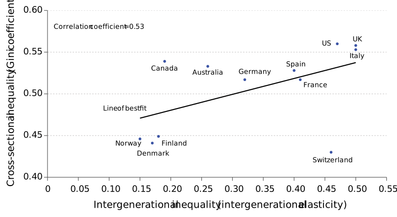
Figure E5.6 Intergenerational and cross-sectional inequality.
Miles Corak. 2013. “Inequality From Generation to Generation: The United States in Comparison”. In The Economics of Inequality, Poverty, and Discrimination in the 21st Century, edited by Robert S. Rycroft. Santa Barbara, CA: Greenwood Pub Group; Wen-Hao Chen, Michael Förster, and Ana Llena-Nozal. 2013. “Globalisation, Technological Progress, and Changes in Regulations and Institutions: Which Impact on the Rise of Earnings Inequality in OECD Countries?” Working Paper Series 597. LIS.
For the countries considered, the figure shows that inequality in earnings at any particular point in time tends to be higher when intergenerational inequality is high. The United States, United Kingdom, and Italy all have both high cross-sectional inequality and high intergenerational inequality. In contrast, both intergenerational inequality and cross-sectional inequality are quite limited in Norway, Denmark, and Finland. Some countries differ according to which type of inequality is more pronounced. Compare, for example, Canada and Switzerland.
Another likely source of the correlation in Figure E5.6 is that in any period (a generation, for example), some individuals experience good luck (for example, living in a region that experienced an economic boom) while others experience bad luck—such as a serious illness (their own or a family member’s), unplanned pregnancy, business failure, or technological change or shifts in demand that made their skills less valuable. These shocks create more inequality in any given generation.

