11.6 Conclusion: Lessons of the model
In this chapter, we saw that employers directly benefit from a firm increasing its profits, but workers usually do not. Workers thus have little incentive to care about increasing a firm’s profits, so long as the firm is earning enough to continue operating. The result is a conflict of interest between workers and employers.
If the employment contract were complete, employers could write it so that workers will get paid only if they exert a certain amount of effort. However, certain features of the employment contract, such as level of effort, length of employment, and unforeseen future tasks, cannot be put into an enforceable contract, making it necessarily incomplete.
The combination of a conflict of interest and an incomplete contract creates a principal–agent problem between the employer (the principal) and the worker (the agent). The employer wants a certain amount of effort from the worker, but the employer cannot directly observe that effort and thus can never be certain how much effort the worker is putting in.
To incentivize workers to provide the effort they require, employers must offer an employment rent, which is the difference in outcome between keeping the job and the workers’ outside option. Key determinants of the employment rent are the wage, personal cost of working, unemployment benefits, other job options, and the unemployment rate. The employment rent must be large enough for the worker to prefer working to shirking. They may get fired if they are caught shirking.
The wage at which a worker will prefer to work instead of risk getting caught shirking is the no-shirking wage. The employer offering the no-shirking wage to the worker is the best-response equilibrium of the principal–agent problem. The no-shirking wage depends not only on the employment rent but also on the extent to which employers monitor their workers. The more a worker is monitored, the more likely they are to get caught shirking. One way employers can reduce the no-shirking wage they must offer is to increase monitoring, though that typically comes with a cost.
The model we developed in this chapter allows us to understand why a particular inefficiency is common to all capitalist economies: the constant existence of unemployment. As we’ve seen, so long as the employment contract is incomplete and employers are unwilling to make workers profit claimants, the cost of job loss needs to be substantial in order to induce sufficient worker effort. With zero or minimal unemployment, such a cost would barely exist. Employers would then lose much of the structural and bargaining power they need if workers are going to put in the effort employers demand. Hence, to remain profitable, employers need unemployment, which makes workers fear losing their jobs enough to exert the effort demanded of them.
Extension 11.6 describes this point in more detail, and Data Extension 11.6 examines which groups suffer most from this feature of capitalism.
Extension 11.6 Why there is always unemployment

Figure E11.3 Unemployment rate in the United States, Spain, Indonesia, Brazil, and South Africa, 1991–2023.
None of these countries, and no capitalist economies, have ever had zero unemployment. Why is there always unemployment in capitalist economies? To answer this question, we first need to distinguish between two types of unemployment: search unemployment and involuntary unemployment.
Two types of unemployment
- search unemployment
- Since workers differ from each other, and so do jobs, unemployed workers and firms with vacancies spend time searching for an employment match that suits them both. Unemployment caused by the search and matching process is called search unemployment.
- involuntary unemployment
- A person is involuntarily unemployed if they are seeking work, and willing to accept a job at the going wage for people of their level of skill and experience, but unable to secure employment.
As we learned in Chapter 10, the labor market is a matching market. If a worker quits a job, it may take some time for that worker to find a new job. When a firm decides to hire a new worker, that process also takes time. The unemployment that results from the time it takes for firms and workers to make a match is search unemployment.
So long as the labor market remains a matching market, there will always be a certain amount of search unemployment. But even if we could eliminate search unemployment, capitalist economies would still have unemployed workers. Even if the matchmaking process could be completed instantaneously, there will always be some workers who want a job, are looking for a job, and are ready to work, but cannot find anything. This type of unemployment is involuntary unemployment.
Whereas search unemployment results from the matching process, involuntary unemployment presents more of a puzzle. It seems inefficient to prevent people who want to work from working. Why does involuntary unemployment happen?
Why employers need unemployment to make profits
So long as the unemployment rate is sufficiently high, workers will expect there to be a significant cost to losing their job. As we saw in this chapter, this expectation produces an employment rent, which incentivizes workers to put in the effort employers demand. Some unemployment is needed if employers want the power to command workers to exert work effort without sharing profits or ownership.
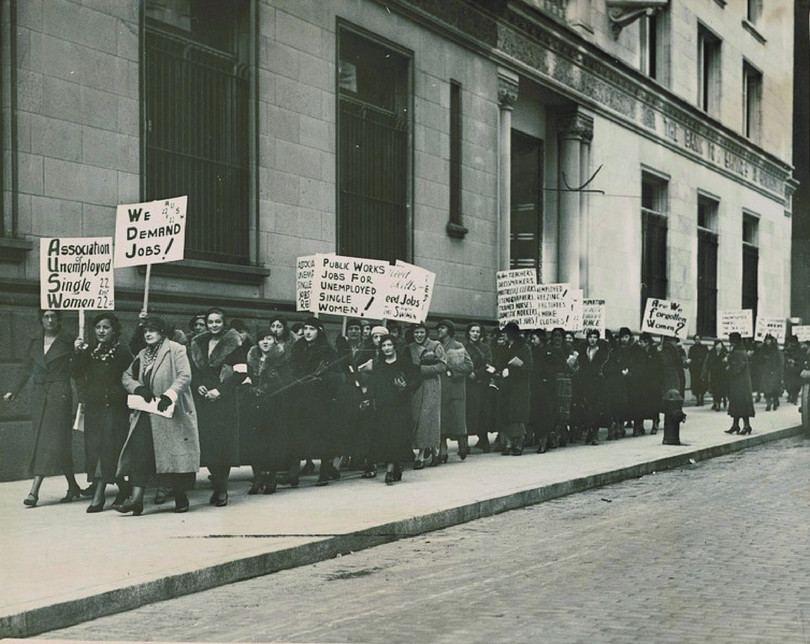
Women march for jobs in New York, 1933. At various points throughout US history, workers have agitated for policies to ensure that anyone who wants a job can get one.
We can see why it is impossible to sustain zero involuntary unemployment in a capitalist economy by thinking through what would happen if there were no involuntary unemployment. Figure E11.4 walks us through each step.
To begin, assume there is zero involuntary unemployment. In this situation, everyone who wants a job right now has one. The only unemployment is search unemployment.
If everyone who wants a job immediately gets one, then losing your job will have basically zero cost. But if the net benefit of your outside option is equal to the net benefit of your current job, there will be zero employment rent. If the workers in a firm have zero employment rent, they have no reason to work. If workers don’t work, then firms cannot produce anything. And if firms cannot produce anything, they will shut down, leading to involuntary unemployment.
Thus, when you start in a situation of zero involuntary unemployment, workers necessarily become involuntarily unemployed. Zero involuntary unemployment is thus not a stable outcome in a capitalist economy.

Figure E11.4 Why zero unemployment is not possible

Zero unemployment

Zero unemployment means there is no cost to losing a job

No cost of job loss means there is no employment rent

With no employment rent, workers put in zero effort

If workers put in zero effort, firms will shut down
Zero unemployment leads to workers becoming unemployed
In other words, involuntary unemployment is necessary in a capitalist economy because without it there is no employment rent, and without employment rent there is no reason for workers in a firm to put in any effort. You can’t have an economy if workers aren’t doing any work.
Exercise E11.7 Search vs. involuntary unemployment
At InnovateTech, some employees are leaving to explore new opportunities, while others take time between jobs to find a good match.
- Define search unemployment and involuntary unemployment using this scenario.
- Why will there always be some level of search unemployment?
- Explain why completely eliminating involuntary unemployment will cause problems for InnovateTech’s owners. What will happen to workers’ motivation and effort if there is no threat of job loss?
Question E11.7
Which of the following is an example of search unemployment? Choose all that apply.
- This is search unemployment—the worker is unemployed while looking for a better match.
- This is voluntary job switching with a short, planned gap, not active search unemployment.
- This is job loss due to firm closure—closer to frictional or structural unemployment depending on circumstances, but not search unemployment by itself.
- This is search unemployment—the graduate is actively looking for a suitable job after graduation.
Data Extension 11.6 Who is unemployed?
In this Data Extension we look at the data on unemployment rates disaggregated by education and then by race. We will use what we’ve learned in this chapter to help us better understand the data.
Education and unemployment
Figure E11.5 shows the US unemployment rate from January 2001 to December 2024 for those over the age of 25 divided into four categories:
- people who never graduated high school
- people who graduated high school and did not take any college classes
- people who attended some college or got an associate’s degree but did not complete a bachelor’s degree
- people who earned at least a bachelor’s degree

Figure E11.5 US unemployment rate for people over the age of 25 by educational outcome, 2001–2024.
US Bureau of Labor Statistics, Unemployment Rate - Less Than a High School Diploma, 25 Yrs. & over, retrieved from FRED, Federal Reserve Bank of St. Louis; Unemployment Rate - High School Graduates, No College, 25 Yrs. & over, retrieved from FRED; Unemployment Rate - Some College or Associate Degree, 25 Yrs. & over, retrieved from FRED; Unemployment Rate - Bachelor’s Degree and Higher, 25 Yrs. & over, retrieved from FRED.
As the figure shows, there is always some unemployment for each of the four categories, but the unemployment levels differ. Comparing the highest and lowest educational levels in the graph, the average unemployment rate over this period was more than three times higher for people who did not graduate high school than for those with at least a bachelor’s degree. Similarly, the average unemployment rate for people with at most a high school degree was about twice the unemployment rate of people with at least a bachelor’s degree.
Figure E11.5 also shows that the size of the unemployment gaps between these groups varies and tends to get smaller when overall unemployment is lower. Between 2009 and 2019, for example, the unemployment rate for people who never graduated college dropped substantially, such that all four lines started to converge around 2019. Lower overall unemployment tends to be especially beneficial for those who typically have the hardest time finding a job.
Why do such gaps exist in the first place? Why do unemployment rates go down as education levels go up? Some key factors include the following:
- On-the-job training: More-educated workers are more likely to take jobs involving more varied and complex tasks. Such jobs tend to require more on-the-job training, because the worker needs to learn about the job to perform it well. More-educated workers thus tend to have more firm-specific assets thanks to the increased on-the-job training they are likely to get. More firm-specific assets lead to higher net benefits of a job, leading to higher average employment rents for more-educated workers, which in turn incentivizes these workers to work harder to keep their job. Because the extra training is costly to the firm, it too has a strong incentive not to fire workers unless it’s absolutely necessary.
- Job search and job offers: Because they often have desk jobs using a computer, more-educated workers are more likely to search for other jobs while they are still employed at their current job, as opposed to waiting until they lose their job to search for another one. More-educated workers are also more likely to receive job offers from other firms while they are employed. Both factors mean that more-educated workers are less likely to have a spell of unemployment between jobs.
- Specialization: Workers who are more highly educated tend to be more specialized, meaning there is a relatively small pool of workers with a given specialization for firms to choose from. Firms will then have to compete more for these workers, who are harder to replace and less likely to be fired.
- Preference for more-educated workers: All else being equal, many employers prefer to hire workers with more education. This is true even for many jobs where a college or high school degree is not necessary, suggesting this preference may have nothing to do with skills. When unemployment is low, some jobs that are usually advertised as requiring a college degree remove that requirement.
Those with higher education also tend to get paid more. In 2024, for example, the median earnings were $2,278 per week for a worker with a PhD, $1,543 per week for a worker with at most a bachelor’s degree, and $930 for a worker with at most a high school diploma. The higher unemployment rates for less-educated workers can help explain these differences. As we saw earlier in this chapter, a higher unemployment rate means a weaker outside option. If the outside option of less-educated workers tends to be weaker, then those workers are going to have lower reservation wages and thus lower no-shirking wages.
Specialization and firm preferences for more-educated workers also tend to push up the wages of more-educated workers, thereby giving them stronger outside options.
Unemployment disaggregated by race
The extent of racial inequality in the labor market is understated in the data because of the large number of Black people who are in prison. As detailed in this article, these individuals are not counted in labor market surveys, and therefore the extent of Black joblessness is understated in the statistics.
Figure E11.6 shows the unemployment rate for white people, Black people, and Hispanic people from January 2001 to December 2024. There are consistent differences in unemployment rates across groups. The unemployment rate for white people is always the lowest, and it is always the highest for Black people. A general rule over this time period is that the unemployment rate for Black people is about twice that of white people. The figure also shows that the unemployment gap between these three racial groups fluctuates with the state of the economy. In 2019 and 2023, for example, unemployment generally was low, and the unemployment rate for the three groups became much closer. By comparison, throughout much of the 1980s, Black unemployment was about 2.5 times that of white unemployment.

Figure E11.6 US unemployment by race, 2001–2024.
US Bureau of Labor Statistics, Unemployment Rate—Black or African American, retrieved from FRED, Federal Reserve Bank of St. Louis; Unemployment Rate—White, retrieved from FRED; Unemployment Rate—Hispanic or Latino, retrieved from FRED.
One reason for these gaps is education. In 2022, 41.8% of white people over the age of 25 had at least a bachelor’s degree, whereas that number was 27.6% for the Black population, and 20.9% for the Hispanic population. Because more education typically leads to lower unemployment rates, racial groups with more education are likely to have lower unemployment, which helps explain why white unemployment is lower than that for Hispanic people and Black people.
For more details on racial differences in education and how they relate to racial segregation, look at this section from the CORE Insight, “Persistent racial inequality in the United States.”
However, differing educational outcomes cannot fully explain the gap in unemployment rates. For one thing, if education alone explained the difference, we would expect Hispanics, who have lower average years of education, to have the highest unemployment rate, which they do not. In addition, if education primarily caused the Black/white unemployment gap, we would expect to see similar unemployment rates for Black workers and white workers who have the same levels of education. Figure E11.7 shows the unemployment rate in 2017 for Black workers and white workers with different levels of education. On the far left, for example, the figure shows the unemployment rate for Black workers and white workers who did not graduate high school. Although both groups have higher unemployment rates than those with more education, the unemployment rate for Black workers with no high school diploma is nearly twice that of similar white workers. A similar pattern is true for every level of education. Education alone cannot therefore explain the overall differences in unemployment between Black workers and white workers.

Figure E11.7 US annual average unemployment by race and education, 2017.
Valerie Wilson. 2018. “50 Years After the Riots: Continued Economic Inequality for African Americans”. Economic Policy Institute.
In Chapter 10 we saw that Black workers and Hispanic workers are more likely to experience labor market discrimination. Figure E11.7 is further evidence of this discrimination: a Black worker with the same education as an equivalent white worker has a harder time finding or keeping employment.
Discrimination affects both unemployment and wages. If a worker expects to face discrimination in the hiring process, then the expected net benefit of their outside option will be lower, because it will take longer to find a job. Their reservation wage and no-shirking wage therefore decrease. Employers may know Black or Hispanic workers have a lower reservation wage, and therefore offer lower wages than they would to similar white workers. The employers’ actions reinforce Black workers’ and Hispanic workers’ expectations of lower pay.
Another cause of the racial gaps in unemployment is segregation. Segregation reduces Black and Hispanic access to employment in two ways: spatial isolation and social isolation. Spatial segregation can impact a worker’s ability to get a job in several ways:
- If a person lives far from areas with high job growth and opportunities, they are less likely to know about job openings in those areas.
- Even if a worker knows about a job opening in the suburbs or a different part of the city, they may not be able to get to that location easily, either because they don’t have a car or because public transit doesn’t exist, doesn’t go to the job’s location, or takes too long.
- Employers located far from Black or Hispanic neighborhoods may be more likely to discriminate against Black or Hispanic workers.
- Black or Hispanic workers may fear venturing into majority white areas.
Compounding the effects of spatial mismatch is the social isolation that results from segregation. As we saw in Chapter 10, when looking for a job, workers use their personal networks—friends, family, friends of friends—to learn about job openings and get hired. Given that racial segregation leads to largely unconnected Black, white, and Hispanic social networks, Black workers and Hispanic workers have a limited capacity to benefit from such practices because Black and Hispanic unemployment rates are higher and white people are more likely to own businesses or be in a strong position to affect hiring decisions.
Exercise E11.8 The education–wage gap: Explaining differences in pay
Using these data from the US Bureau of Labor Statistics on the median weekly earnings for full-time workers disaggregated by educational outcome, answer the following questions.
- What do the data suggest about the relationship between workers’ education and their wage?
- Using what you’ve learned, what might explain the wage gaps you observe between workers with different levels of education?
- Have the wage gaps between workers with different educational levels changed over time? If so, how? What might explain these changes? If there were no changes, why do you think they stayed the same?
Question E11.8
Which of the following is a reason why college-educated workers have a lower unemployment rate than those with only a high school degree? Choose all that apply.
- The difference is not explained by work ethic, but by labor market factors.
- More-educated workers are often in specialized fields, making them harder to replace and less likely to be laid off.
- Many employers prefer more-educated workers even for jobs that don’t require a degree, giving those workers stronger employment prospects.
- More-educated workers generally earn higher wages, not lower wages.
Skills and learning objectives
- defining terms
- translating a story into an abstract model
- adjusting a model in response to economic or institutional changes
- using a game tree
- reading a flow chart
- reading comprehension (difficult material)
Concepts to be learned
- conflicts of interest between employers and workers
- incomplete employment contract
- principal–agent problem
- employment rent and the cost of job loss
- no-shirking wage
- search and involuntary unemployment
Seeing the Principles in Action
| Principle | Example | Everyday economics |
|---|---|---|
| Interdependence principle | As owners of a Mexican restaurant, you and your partner depend on the effort of workers like Celia to earn a profit, and Celia depends on the wage you offer to earn an employment rent. | Think about a job you or someone you know has had at a firm. How did the profits earned by the employer depend on the workers’ effort? Did the employer need to offer a large employment rent to motivate workers to put in effort? Why or why not? |
| Doing the best you can principle | You and your partner do the best you can by paying Celia as little as possible for the effort you need from her. Celia does the best she can by maximizing her wage and minimizing her effort. | Think about a job you have had. Did you try to figure out the lowest amount of effort you could exert without losing your job? Did you shirk or consider doing so? How did your employer try to prevent you from shirking? |
| Rules of the game principle | During the COVID-19 pandemic, the federal government altered the rules of the game by increasing unemployment benefits by $600 per week, which changed workers’ reservation and no-shirking wages. | What other formal and informal institutions affect workers’ no-shirking wages? Can you think of any examples of major institutional changes in the United States that affected the outcomes of workers and employers? |
| Trade-offs and opportunity costs principle | Celia faces a trade-off between working (which means keeping her job but incurring cost of working) and shirking (which provides a better outcome for her but comes with the risk of getting caught shirking and losing her job). | Think about any employers you know. How do they navigate the trade-off between the increased effort that comes from paying their workers more and maximizing their profits? If you were an employer, how would you go about setting wages? |
| Principle of gains from cooperation and conflict of interest | You, your partner, and Celia all experience gains from cooperation, because you and your partner can earn profits and Celia earns an employment rent. But there is a conflict because a higher employment rent for Celia decreases your profits. | If you’ve had a job, have you ever had a conflict with your employer over something that affected your employment rent? What was the conflict about? How was that conflict addressed? How would you have acted if you had been the employer? |
| Principle of individual and societal interests | Employers doing the best they can in a capitalist economy leads to some workers being involuntarily unemployed, which hurts those workers and is inefficient for society as a whole. | Have you or anyone you know ever been involuntarily unemployed? How did that unemployment affect their well-being and overall economic outcome? How might policy changes help those who are involuntarily unemployed? |
References
Atkin, D., A. Chaudhry, S. Chaudry, A. K. Khandelwal, and E. Verhoogen. 2017. “Organizational Barriers to Technology Adoption: Evidence From Soccer-Ball Producers in Pakistan”. The Quarterly Journal of Economics 132(3): pp. 1101–1164.
Bewley, T. F. 1999. Why Wages Don’t Fall During a Recession. Harvard University Press.
Bowles, S., 1985. “The Production Process in a Competitive Economy: Walrasian, Neo-Hobbesian, and Marxian Models”. The American Economic Review 75(1): pp. 16–36.
Bowles, S., 2006. Microeconomics: Behavior, Institutions, and Evolution. Princeton University Press.
Brown, M., A. Falk, and E. Fehr. 2004. “Relational Contracts and the Nature of Market Interactions”. Econometrica 72(3): pp. 747–780.
Cairó, I., and T. Cajner. 2018. “Human Capital and Unemployment Dynamics: Why More Educated Workers Enjoy Greater Employment Stability”. The Economic Journal 128(609): pp. 652–682.
Coase, R. H., 1992. “The Institutional Structure of Production”. American Economic Review 82(4): pp. 713–719.
Coase, R. H., 1937. “The Nature of the Firm”. Economica 4(16): pp. 386–405.
Couch, K. A., and D. W. Placzek. 2010. “Earnings Losses of Displaced Workers Revisited”. American Economic Review 100(1): pp. 572–589.
Coviello, D., E. Deserranno, and N. Persico. 2022. “Minimum Wage and Individual Worker Productivity: Evidence From a Large US Retailer”. Journal of Political Economy 130(9): pp. 2315–2360.
Davis, S. J., and T. von Wachter. 2011. “Recessions and the Costs of Job Loss”. Brookings Papers on Economic Activity. 2011(2): p. 1.
Hansmann, H., 2000. The Ownership of Enterprise. Belknap Press.
Farber, H. S., D. Herbst, I. Kuziemko, and S. Naidu. 2021. “Unions and Inequality Over the Twentieth Century: New Evidence From Survey Data”. The Quarterly Journal of Economics 136(3): pp. 1325–1385.
Helper, S., M. Kleiner, and Y. Wang. 2010. “Analyzing Compensation Methods in Manufacturing: Piece Rates, Time Rates, or Gain-Sharing?” NBER Working Papers No. 16540, National Bureau of Economic Research.
Hussam, R., E. M. Kelley, G. Lane, and F. Zahra. 2022. “The Psychosocial Value of Employment: Evidence From a Refugee Camp”. American Economic Review 112(11): pp. 3694–3724.
Jacobson, L., R. L. Lalonde, and D. G. Sullivan. 1993. “Earnings Losses of Displaced Workers”. The American Economic Review 83(4): pp. 685–709.
Jäger, S., C. Roth, N. Roussille, and B. Schoefer. 2024. “Worker Beliefs About Outside Options”. The Quarterly Journal of Economics 139(3): pp. 1505–1556.
Kalecki, M., 1943. “Political Aspects of Full Employment”. The Political Quarterly 14(4): pp. 322–330.
Kletzer, L. G., 1998. “Job Displacement”. Journal of Economic Perspectives 12(1): pp. 115–136.
Kroszner, R. S., and L. Putterman (eds.). 2009. The Economic Nature of the Firm: A Reader (3rd ed.). Cambridge University Press.
Lazear, E. P., K. L. Shaw, and C. Stanton. 2016. “Making Do With Less: Working Harder During Recessions”. Journal of Labor Economics 34(1/2): pp. 333–360.
Manning, A., 2003. Monopsony in Motion: Imperfect Competition in Labor Markets. Princeton University Press.
Mincer, J., 1991. “Education and Unemployment”. NBER Working Paper.
Newman, K. S., and E. S. Jacobs. 2023. Moving the Needle: What Tight Labor Markets Do for the Poor. University of California Press.
Oh, S. 2023. “Does Identity Affect Labor Supply?” American Economic Review 113(8): pp. 2055–2083.
Pencavel, J. 2002. Worker Participation: Lessons From the Worker Co-ops of the Pacific Northwest. Russell Sage Foundation Publications.
Pierce, L., et al. 2013. “Cleaning House: The Impact of Information Technology Monitoring on Employee Theft and Productivity”. SSRN Electronic Journal.
Rose, E. K., and Y. Shem-Tov. 2023. How Replaceable Is a Low-Wage Job? (No. w31447). National Bureau of Economic Research.
Rosenfeld, J. 2021. “You’re Paid What You’re Worth: And Other Myths of the Modern Economy”. In You’re Paid What You’re Worth. Harvard University Press.
Ruffini, K. 2024. “Worker Earnings, Service Quality, and Firm Profitability: Evidence From Nursing Homes and Minimum Wage Reforms”. Review of Economics and Statistics 106(6): pp. 1477–1494.
Semuels, A., 2009. “Productivity Rises as Workers Do More With Less”. Los Angeles Times.
Simon, H. A. 1951. “A Formal Theory of the Employment Relationship”. Econometrica 19(3): pp. 293–305.
The Economist. 2012. “The Feeling Is Mutual”. January 21.
Thiel, C., et al. 2022. “Monitoring Employees Makes Them More Likely to Break Rules”. Harvard Business Review.
Toynbee, P. 2003. Hard Work: Life in Low-Pay Britain. Bloomsbury Publishing.
Weil, D. 2014. The Fissured Workplace. Harvard University Press.
Williamson, O. E. 1985. The Economic Institutions of Capitalism. Collier Macmillan.
Education Pays, 2024: Career Outlook. US Bureau of Labor Statistics, May 2025.
