13.3 Shaping demand

In Chapter 12, we learned that firms do the best they can to generate as much profit as possible. In the CORE Brewing Co. example, you compared the additional revenue from selling one more keg of beer (marginal revenue) to the additional cost of producing that keg (marginal cost), and you set the price where the two were equal. We saw that following this rule of thumb allows firms to maximize profit.

Figure 13.5 (A) revisits CORE Brewing Co.’s demand curve, marginal revenue curve, and marginal cost curve from Chapter 12. In that scenario, you charged $240 for a keg of beer and produced 4 kegs per day. This price and quantity combination gave you the highest possible profit, based on the demand you faced and your costs of production. The black arrow shows how much the price exceeds the unit cost—this is your markup, which indicates how much profit you earn on each keg sold.

Panel (B) shows an alternative situation for CORE Brewing Co., with a different demand curve, marginal revenue curve, and marginal cost curve. Let’s compare the two panels:

• The demand curve in panel (B) is steeper than the demand curve in panel (A). The steeper demand curve represents less elastic demand.
• At a quantity of 4 kegs per day, the price is $240 in panel (A), but $320 in panel (B).
• The markup bracket in panel (B) shows a greater difference between price and cost per unit.
• The green profit area is larger in panel (B), meaning higher overall profits.

As a brewer, which situation would you prefer for CORE Brewing Co.: panel (A) or panel (B)?

Fullscreen

https://books.core-econ.org/uoe-101/13-03.html#figure-13-5

Demand, marginal revenue, and marginal costs for CORE Brewing Co.’s beer

Figure 13.5 Demand, marginal revenue, and marginal costs for CORE Brewing Co.’s beer Panel (A) shows CORE Brewing Co.’s demand curve from Chapter 12. In panel (A), CORE produces 4 kegs of beer per day and charges $240 per keg when it sets MR = MC to maximize its profits. Panel (B) shows a steeper demand curve for CORE Brewing Co. In panel (B), CORE produces 4 kegs of beer per day and charges $320 per keg when it sets MR = MC. The steeper curve is relatively less elastic.

Fullscreen

https://books.core-econ.org/uoe-101/13-03.html#figure-13-5a

Costs, markup, and profit of the flatter demand curve

Let’s start with Figure 12.8 from Chapter 12, which showed us the price that CORE Brewing charges and the amount of beer it produces when it maximizes its profit (which it chose by setting MR = MC). The figure also showed us CORE Brewing’s profits and total costs. We have changed the range of the vertical axis, increasing it from 440 to 600 for comparison with the demand curve shown in panel B.

Fullscreen

https://books.core-econ.org/uoe-101/13-03.html#figure-13-5b

Calculating the slope of the flatter demand curve

We described the demand curve for CORE Brewing in Figure 12.8 as ‘flatter’. To compare it to the new demand curve in panel (B), let’s calculate the slope of the flatter demand curve. We calculate the slope by finding the rise over the run, or the change in \(y\) (\(\Delta y\)) over the change in \(x\) (\(\Delta x\)). Comparing its vertical intercept of price = $400 when quantity sold = 0 to when it charges a price of 0 and its quantity sold is 10 kegs, the change in \(y\) = –400. Price decreases from $400 to $0, and therefore the change in \(y\) is negative. The change in \(x\) = 10 (kegs sold increase from 0 to 10), and therefore the change in \(x\) is positive. Thus the slope is \(\text{slope} = \frac{\Delta y}{\Delta x} = \frac{-400}{10} = - 40\). This flatter and relatively more elastic demand curve means that for each change in price, the quantity demanded changes more than on another demand curve (such as the demand curve in panel B).

Fullscreen

https://books.core-econ.org/uoe-101/13-03.html#figure-13-5c

Costs, markup, and profit of the steeper demand curve

Let’s now look at a demand curve and a marginal revenue curve that are steeper than CORE Brewing’s original demand curve. The figure shows this steeper demand curve (shown in lighter blue), which is more inelastic than the original curve. Because the firm faces a downward-sloping demand curve, it must lower its price to sell an additional keg of beer. This lower price applies not just to the extra keg, but to all kegs sold. As a result, the additional revenue gained from selling one more keg (marginal revenue) is less than the price charged, causing the marginal revenue curve to be steeper than the demand curve. CORE Brewing chooses its output (kegs of beer) where its marginal cost equals its marginal revenues at point I′, or a quantity of 4 kegs. At 4 kegs, CORE Brewing charges a price of $320, shown by point H′. Because CORE Brewing faces both marginal costs and fixed costs of production, its average cost of producing 4 kegs of beer is shown at point J′ where average total costs are $105. With a price of $320 and average total costs of $105, CORE Brewing Co.’s markup is $215 on the steeper demand curve. Its total costs are $420 and its economic profits are therefore $860 on the steeper demand curve.

Fullscreen

https://books.core-econ.org/uoe-101/13-03.html#figure-13-5d

Calculating the slope of the steeper demand curve

We described the new demand curve for CORE Brewing as ‘steeper’. To compare it to the old demand curve in panel (A), let’s calculate the slope of the steeper demand curve. We calculate the slope by finding the rise over the run, or the change in \(y\) (\(\Delta y\)) over the change in \(x\) (\(\Delta x\)). Comparing its vertical intercept of price = $560 when quantity sold = 0 to when it charges a price of 0 and its quantity sold is 9.33 kegs, the change in \(y\) = –560. Price decreases from 560 to 0, and therefore the change in \(y\) is negative. The change in \(x\) = 9.33 (kegs sold increase from 0 to 9.33, and therefore the change in \(x\) is positive). Thus the slope is \(\text{slope} = \frac{\Delta y}{\Delta x} = \frac{-560}{10} \approx - 60\). This steeper and relatively more inelastic demand curve means that for each change in price, the quantity demanded changes less than on another demand curve (such as the demand curve in panel A).

Fullscreen

https://books.core-econ.org/uoe-101/13-03.html#figure-13-5e

Comparing the slopes and profits of the flatter demand curve and the steeper demand curve

This figure compares the profits of the steeper demand curve and the flatter demand curve. When the demand curve is steeper, demand is relatively more inelastic and profits will be higher because CORE Brewing can charge more for a keg of beer. The steeper demand curve results in greater profits ($860) than the flatter demand curve ($540), so profits are $320 higher when demand is relatively more inelastic. This scenario might occur if CORE Brewing spent more money on advertising to show beer drinkers how unique its beer is relative to its competitors, or because CORE Brewing advertised its commitment to the environment. Some buyers are willing to pay more for products produced by firms that are committed to operating in sustainable ways.

You might prefer the scenario in panel (B) because you can charge a higher price, which is possible because the demand curve in panel (B) shows that buyers are willing to pay more for your beer. The greater steepness of the demand curve in panel (B) suggests that demand is less elastic than in panel (A)—that is, buyers are less responsive to changes in price. This is why the markup—the difference between price and cost—is higher in panel (B). When buyers are less sensitive to price, you can charge a higher markup. Panel (B) represents a situation where CORE Brewing has greater market power and earns more profit per unit than it would under the demand conditions in panel (A).

Now suppose that panel (A) reflects CORE Brewing’s current situation. Can the firm pursue any strategies to shift itself closer to the scenario in panel (B)? The answer is yes. Firms can take several steps to create conditions where:

• demand for their product becomes less elastic,
• buyers are more willing to pay higher prices, and
• the markup is larger.

interdependence principle, principle of interdepence

The outcomes people obtain in economic interactions depend on the actions that they and others take in response to each other and on what they believe about the future.

principle of trade-offs and opportunity cost

The gains you make by choosing some action typically come at the cost of gains that would have been possible had you acted differently.

In the next sections, we explore three common strategies that firms use to increase market power and reduce price elasticity of demand: advertising, product differentiation, and reducing the number of competitors. The interdependence principle reminds us that economic outcomes are shaped by the actions of many different people and firms, often acting independently. This principle is especially relevant here, as the success of these strategies depends not only on the firm’s own decisions but also on how buyers, competitors, and the government respond.

At the same time, the trade-offs and opportunity costs principle reminds us that choosing one course of action means giving up another. For example, if a firm invests heavily in an advertising campaign to promote its brand or highlight unique product features, it may succeed in making buyers more loyal and less price-sensitive. However, the resources spent on advertising could have been used for other valuable activities, such as expanding production capacity or adopting new technology. Firms must weigh these trade-offs carefully when deciding how much to strengthen their market power.

Advertising

Advertising is a strategy widely used by firms that produce differentiated products. Its main goal is to convince buyers that fewer close substitutes are available. If a firm can successfully persuade buyers that its product is unique, buyers will be less sensitive to price changes, allowing the firm to charge higher prices. For example, from 2006 to 2009, Apple ran its Get a Mac campaign, which featured actors rather than actual computers to personify the differences between Macs and PCs. By emphasizing how Macs were distinct and superior, Apple aimed to convince buyers that PCs were not good substitutes for Macs, strengthening Apple’s market power and allowing it to set higher prices.

Fullscreen

https://books.core-econ.org/uoe-101/13-03.html#figure-13-6

Figure 13.6 Share of US firms that use influencers for marketing purposes.

Christopher Ross. 2025. Influencer Marketing Penetration Rate in the U.S. 2020–2025. Statista.

Social media, and particularly social media influencers, have become a popular way for firms to advertise and enhance brand loyalty. Social media influencers range from celebrities and content creators to college students and working professionals. Nano-influencers have anywhere from 1,000 to 10,000 followers, while mega-influencers have over a million followers. Some influencers are paid a fee to promote a product, while others receive free products for their endorsements or simply recommend the brands they like without any connection to a firm. Figure 13.6 shows the growing role of influencers in marketing. As of this writing, it is estimated that 86% of companies market their products using social media influencers.

Influencers use platforms such as Instagram, YouTube, Facebook, and TikTok to promote brands and encourage buyers to purchase specific products. Because they have already established trust and credibility among their followers, influencers are sometimes in a better position than the firm to engage with and influence buyers. Responses from the Pew Research Center’s 2022 survey of adults show that 41% of adults between the ages of 18 and 29 purchased a product after seeing an influencer’s post about it on social media.

Data Extension 13.3 Advertising and market power

In 2023, market analysts Schonfeld and Associates estimated that advertising on breakfast cereals in the United States was about 4.45% of total sales revenue of those cereals. Figure E13.10 shows the relationship between market share and advertising expenditure for the best-selling breakfast cereal brands in the Chicago area in 1991 and 1992. For breakfast cereals, market share was not closely related to price. But it is clear from Figure E13.10 that the brands with the highest share were those that spent the most on advertising. For example, the market share for GM’s Cheerios was 4.4% and the company spent $7.3 million on advertising. Analyzing cereal purchases in Chicago with this dataset, Matthew Shum, an economist, showed that advertising was more effective than price discounts in stimulating demand for a brand. Because brands that were already well known spent the most on advertising, he concluded that advertising’s main function is not to inform consumers about the product, but rather to increase brand loyalty and encourage consumers of other cereals to switch.¹

Fullscreen

https://books.core-econ.org/uoe-101/13-03.html#figure-e13-10

Figure E13.10 Advertising expenditure and market share of breakfast cereals in Chicago, 1991–1992.

Figure 1 in Matthew Shum. 2004. “Does Advertising Overcome Brand Loyalty? Evidence From the Breakfast-Cereals Market”. Journal of Economics and Management Strategy 13(2): pp.  241–72. The analysis includes the top 50 brands of cereals from Kelloggs, General Mills, Post, Ralston, and Quaker Oats.

However, as more and more firms increase their advertising spending, it becomes less likely that any single firm will see a significant boost in market share from additional advertising. When all firms are competing for attention, the impact of one firm’s efforts may be diluted by the similar efforts of others.

Data Extension 13.3a Environmental consequences of digital advertising

Digital advertising is the use of online channels, platforms, and technologies to promote products, services, or brands to buyers. In addition to appearing in television commercials or newspapers, ads now appear on search engines like Google, social media platforms like TikTok, streaming services such as YouTube, and within apps and mobile games. Digital advertising often uses data and algorithms to target specific audiences based on demographics, online behavior, or interests. This is why you might see an Adidas ad appear in your Instagram feed after you searched for cool running shoes. Figure E13.11 shows that since 2022, firms have spent more on digital advertising than on television ads.

Fullscreen

https://books.core-econ.org/uoe-101/13-03.html#figure-e13-11

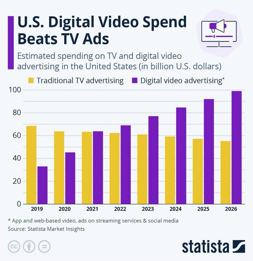
Figure E13.11 US Digital video spending beats TV ads.

Katharina Buchholz. 2024. U.S. Digital Video Spend Beats TV Ads. Statista.

Each online ad, especially video content, requires storage and delivery from data centers and servers that consume electricity. Many of these data centers rely on fossil fuels, contributing to greenhouse gas emissions. Figure E13.12 illustrates that digital advertising campaigns can generate more carbon emissions than the average person produces in a year.

Fullscreen

https://books.core-econ.org/uoe-101/13-03.html#figure-e13-12

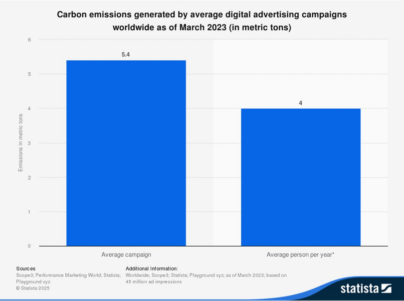
Figure E13.12 Carbon emissions generated by average digital advertising campaigns worldwide, March 2023.

Emissions Generated by Digital Ad Campaigns 2023. Statista. June 27, 2025.

As discussed earlier in the chapter, when many firms increase their advertising spending at the same time, it becomes less likely that any one firm will see a significant boost in market share from additional ads. When all firms are competing for attention, the effect of one firm’s advertising is often offset by the similar efforts of others. Beyond the environmental damage, excessive ad spending can also divert resources away from other valuable uses, such as improving products, investing in innovation, lowering prices, or providing better customer service.

If rival firms continue to escalate their spending on digital advertising without gaining a competitive edge, the result is wasted financial resources, lost opportunities for more productive investments, and unnecessary environmental harm.

Product differentiation

Fullscreen

https://books.core-econ.org/uoe-101/13-03.html#figure-13-7

Figure 13.7 Market share of online dating apps.

Stacy Jo Dixon. 2025. Digital Market Outlook: Global Dating Services Market Share 2022. Statista.

Consider the market for dating apps, such as Tinder, Bumble, Hinge, Grindr, and dozens of other smaller competitors (Figure 13.7). With so many different dating apps available, each firm tries to convince users that their dating app is distinct from or superior to other dating apps. In other words, they want to convince users that few substitutes exist for their app. For example, eHarmony is a dating app for people who want to get married, Uniform Dating is an app for people with jobs that require wearing a uniform, Raya is an exclusive, members-only dating app (individuals need to submit an application and receive approval to participate), and Tinder was the first to create the left–right swipe feature. Women-founded and women-focused Bumble attempts to distinguish itself from other dating apps by creating a safe and empowering environment for women. For example, Bumble allows women to initiate conversations to give them greater control over conversations. In addition, Bumble has invested in research to develop enhanced safety features. For example, the firm developed a Private Detector that automatically detects, blurs, and warns users when they might receive a lewd photo.

By emphasizing their unique features, dating apps hope to reduce their price elasticity of demand, making users less likely to switch to alternative apps. However, investing in differentiation means that dating app companies have fewer resources to allocate to other areas of their businesses. They must weigh these trade-offs and pursue differentiation strategies only up to the point where the benefits outweigh the opportunity costs.

Reducing the number of competitors

Another strategy that firms use to make their demand less elastic is to create barriers to entry for new firms trying to enter the market. Sometimes barriers to entry are called “moats” because, like the protective water barriers around old castles, they protect the existing firms from intrusion by “outsiders.”

A castle with a water-filled moat surrounding it.

In 2023, the Federal Trade Commission, the US federal agency that enforces consumer protection and antitrust laws, along with 17 US states, sued Amazon, alleging that the firm uses strategies to prevent rival firms from growing and new firms from entering the market. For example, third-party sellers that sell their products at lower prices on non-Amazon sites might see their products demoted in search results on Amazon.com. So, for example, if Hydro Flask wants to sell its water bottles at a lower price on its own website, Amazon might retaliate by making sure that Hydro Flask water bottles are not the first water bottles that Amazon.com shoppers see when searching for water bottles. Instead, Hydro Flask water bottles will not be shown until the second or third page of a buyer’s search.

predatory pricing

Predatory pricing occurs when an incumbent firm charges a price lower than its marginal costs, seeking to drive its competitors out of business.

economies of scale

When production exhibits increasing returns to scale, increasing all of the inputs to a production process by the same proportion increases the output by a higher proportion.

Amazon has also been accused of selling its smart home devices (for example, Alexa devices) at prices below the cost of producing them as a way to keep other firms, such as Google (with its “Hey Google” devices), from entering the market for home devices. This practice is known as predatory pricing. By lowering its prices below the marginal costs of producing them, Amazon generates losses for itself on that particular product line, but also undercuts its competitors and grows its Alexa network of users. By selling smart home devices at low prices, Amazon encourages voice shopping and personalized product recommendations. The expanding network also generates valuable buyer data, helping Amazon to better target buyer preferences.

Both of these strategies create less elastic demand for Amazon, which means that buyers are more likely to purchase from Amazon and pay the prices posted by Amazon. If Amazon decides to raise prices, it will lose some buyers, but not very many, because it is the largest e-commerce market.

Amazon also benefits from economies of scale, which we introduced in Chapter 4. Economies of scale occur when a firm’s average total costs fall when the firm becomes larger. For example, Amazon—an enormous company—can negotiate lower prices from its suppliers, which allows it to sell products at lower prices. Amazon’s sheer size makes it challenging for any new firms to enter the e-commerce market and for existing firms to expand. For example, think about Target, which competes with Amazon. The size of Amazon and the number of buyers who purchase products from Amazon.com can make it hard for Target to sell its products on Target.com. As a result, Amazon faces fewer competitors, making the demand for its products less elastic and giving it more power to set prices higher. In other words, economies of scale can reduce the number of competitors.

When firms adopt strategies to make the demand for their products less elastic, they can charge a higher price. In addition, adopting these strategies has implications for rival firms. For example, advertising, economies of scale, and predatory pricing make Amazon’s demand less elastic, but those same strategies make the demand curve for rivals such as Target more elastic. In other words, these strategies help Amazon charge higher prices, but its rivals will have fewer opportunities to charge higher prices.

In the next two sections, we explore how market power affects the distribution of the benefits from exchange between buyers and sellers.

Data Extension 13.3b Economies of scale and market power

Decreasing average costs limits competition by limiting the number of producers that can participate profitably in the market. Consumer demand is fulfilled by a small number of firms operating at a large scale, lowering their costs per unit and leaving no opportunities for potential competitors.

When firms have strongly decreasing average costs, competition tends to be winner-takes-all. The first to exploit the cost advantages of large size prevents other firms from succeeding and, as a result, limits competition. For example, in the market for internet search engines, Google established the technological infrastructure and expertise to meet the needs of a large number of users, and the more searches it conducted, the more data it gathered, lowering its costs of serving other users.

network economies of scale

These exist when an increase in the number of users of an output of a firm implies an increase in the value of the output to each of them, because they are connected to each other.

Figure E13.13 shows some examples of US markets dominated by a small number of firms. Strongly decreasing average costs are an important factor in several industries, such as internet searches, dominated by Google. Similarly, wireless carriers (mobile phone networks) have large fixed infrastructure costs, and just four providers dominate the US market. Another factor, particularly in the case of social media platforms such as Facebook and YouTube, is the benefit from network economies of scale.

Several measures are used to determine market share for the industries in Figure E13.13. For digital companies, the most common measures of market power and costs may not present an accurate picture. For example, some products are free to customers, meaning that revenue from end users is not a useful measure. Similarly, employment may not be a strong indicator of costs. Focusing on usage—for example, the number of searches on a browser, the number of users, or the number of visits to a social media platform—can provide a better comparison of scale.

Fullscreen

https://books.core-econ.org/uoe-101/13-03.html#figure-e13-13

Figure E13.13 Economics of scale and market share.

J. Shambaugh, R. Nunn, A. Breitwieser, and P. Liu. 2018. “The State of Competition and Dynamism: Facts About Concentration, Start-ups, and Related Policies”. Hamilton Project. Washington, DC: Brookings Institution.