13.2 How do buyers respond to price changes?
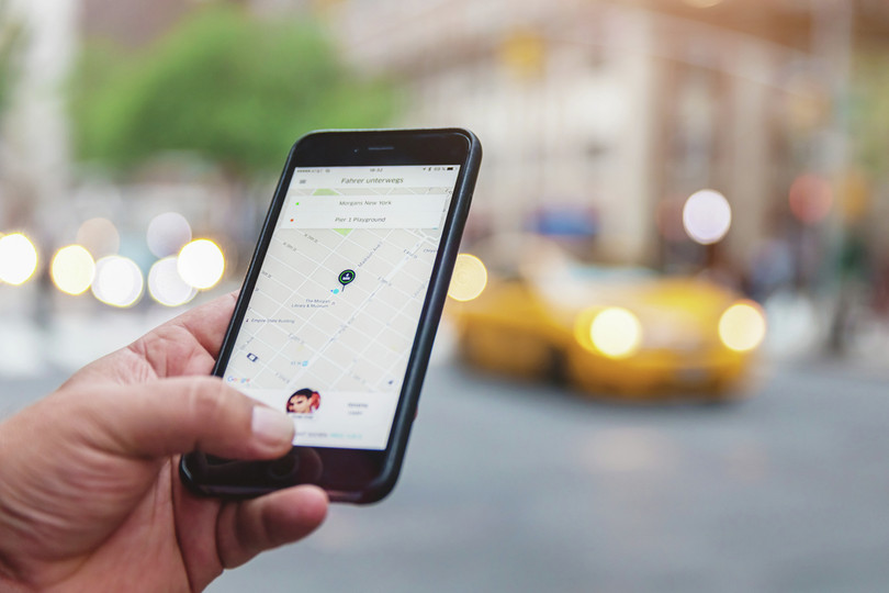
Buyers can arrange for ride service using the Uber app.
Imagine it is a hot afternoon, and you walk to a campus vending machine to buy a cold drink. You notice that the price of your favorite drink is higher than it was earlier that morning when temperatures were cooler. How would you respond to the price increase? Would you still buy the drink?
In 1999, Coca-Cola bet that you would. The company began testing temperature-sensitive vending machines that raised the price of a can of Coke when it was hot and lowered the price when it was cooler. The experiment didn’t sit well with consumers. Many Coke drinkers saw it as unfair, and the backlash was strong enough that Coca-Cola abandoned the temperature-based pricing model.
Fast-forward to today, when Uber uses a similar pricing approach with its surge pricing system. By analyzing real-time data, Uber raises prices above the base fare when demand for rides exceeds the number of available drivers. As a result, ride prices can change quickly, sometimes within minutes. Because Uber tracks which fares riders accept or reject, the company gains valuable insight into how customers respond to price changes.
- price elasticity of demand
- The price elasticity of demand is a measure of buyers’ responsiveness to a price change.
When Uber first introduced surge pricing, riders reacted much like Coke drinkers did—they hated it. But, unlike Coca-Cola, Uber stuck with its dynamic pricing model. Economists have used Uber’s rich data to estimate how responsive riders are to changes in prices, and their research shows that riders don’t respond much to price changes. In other words, when surge pricing goes into effect and prices are higher, Uber loses some riders, but not very many. Economists call buyers’ responsiveness to price changes the price elasticity of demand.
Firms prefer to charge higher prices, but only if doing so doesn’t drive away too many potential buyers, which would reduce their economic profits. Understanding how buyers respond to price changes helps firms do the best they can by determining how high they can set prices without losing too much business. Firms that sell to buyers who do not respond much to higher prices can increase their markups and therefore have greater market power.
Data Extension 13.2 Pricing with algorithms

Algorithms.
On January 22, 2020, gunfire erupted outside a McDonald’s in downtown Seattle, killing one person and injuring seven others, including a nine-year-old boy. As people tried to flee downtown Seattle, Uber and Lyft fares surged up to five times the normal rates due to the greater demand for rides. The prices remained high for about an hour after the incident, at which point Uber and Lyft manually shut down their surge pricing (Baruchman and Clarridge, 2020; Soper 2020). While Uber began capping its surge pricing during emergencies in 2014, fares still surged immediately after the Seattle shooting, angering many riders.
Marketing professors Marco Bertini and Oded Koenigsberg argue that pricing algorithms lack “the empathy required to anticipate and understand the behavioral and psychological effects that price changes have on customers.” (Bertini and Koenigsberg, 2021) They suggest that firms such as Uber should develop “a faster response or a more proactive mechanism for preventing the soaring prices” during emergencies.
Economists have also shown that pricing algorithms can result in higher prices for buyers. To illustrate how this happens, let’s set up a game based on the following rules:
- Players: There are two firms, Firm A and Firm B. Firm A has access to a fast, high-powered pricing algorithm while Firm B does not have access to such an algorithm.
- Order of play: Firm B sets its price and then Firm A sets its price in response to Firm B’s price.
- Actions: To gain a greater share of the market, each firm will charge $4 less than its competitor. For example, if Firm B charges $25, then Firm A will set its price at $21. The only difference is that Firm A uses a pricing algorithm and programs it to automatically set the price $4 lower than Firm B’s price. Firm B doesn’t use an algorithm and has to set the price manually after observing Firm A’s price.
- Payoffs: The payoff is the profit that is generated based on the prices that each firm sets given the price set by its competitor.
Suppose that we start with Firm B charging a price of $20 (Figure E13.6). To gain more market share, Firm A programs its algorithm to set its price $4 lower than Firm B’s price. This means that Firm A will charge a price of $16. Firm A could also keep the price the same as Firm B’s, but it wants to lower its price by $4 to attract more buyers. Because Firm A now has the lower price, it realizes greater profits. Firm B gathers data and notices the lower price that Firm A now charges. Firm B can either keep its price of $20 and let Firm A gain more buyers, or it can lower its price by $4 to a price of $12 (that is, $4 lower than Firm A’s price of $16). Firm B decides to lower its price because it doesn’t want to lose all its buyers to Firm A. Now Firm A’s algorithm immediately detects Firm B’s price cut to $12, and it sets Firm A’s price to $8. Some might argue that this lower price is great for buyers because the price keeps getting lower and lower, but economists Zach Brown and Alexander MacKay use hourly prices for over-the-counter allergy drugs from five online retailers to show that this is not what happens.

Figure E13.6 Will pricing algorithms result in lower prices or higher prices?
This figure illustrates a sequential game in which Firm A sets its price based on the price set by Firm B and vice versa. Each firm adopts a price strategy where price is set at $4 less than the price set by its competitor. The only difference is that Firm A uses an algorithm that can react immediately, and Firm B adjusts its price only after it has obtained data on its competitor’s pricing strategies.
Firm B knows that Firm A has a fast and reliable algorithm that will always lower the price within seconds of Firm B lowering its price. In other words, Firm B will never have a long enough moment to gain buyers and realize higher profits from its lower price. It will always be beaten by Firm A’s quick algorithm. Brown and MacKay show that Firm B will actually benefit more from charging a very high price from the very beginning to take into account Firm A’s algorithm. Thus, buyers end up paying a lot more for the product because Firm B anticipates what Firm A’s algorithm will do. To prevent higher prices for buyers, Brown and MacKay suggest that policymakers limit firms’ ability to set prices based on their rivals’ prices or limit the number of times per day that prices are allowed to change.

Computer algorithms deciding on prices.
Economists Emilio Calvano, Giacomo Calzolari, Vincenzo Denicolò, and Sergio Pastorello (2020) show that prices may be higher for buyers when algorithms are used. They programmed two algorithms to compete with each other to measure the likelihood that the algorithms could end up tacitly colluding with each other on price. The algorithms were programmed to learn through trial and error, such as learning how to punish each other when prices are set low. The researchers showed that instead of setting prices low to compete with each other, the algorithms ended up tacitly colluding to set high prices.
While technology has made it easier for firms to set their prices, it is not clear that buyers always benefit.
The demand curve and buyers’ responsiveness to changes in price
Figure 13.3 shows two possible downward-sloping demand curves for a fictional firm called Aqua, which produces reusable water bottles similar to those made by Hydro Flask, Stanley, and S’well. In panel (a), the firm’s demand curve is relatively steep. In panel (b), the demand curve is relatively flat. Both curves slope downward, reflecting the fact that water bottles are a differentiated product and that quantity demanded increases as price decreases. Aqua’s bottles, for example, have unique features such as the ability to keep drinks cold for three days and a notification system that alerts users to hydrate if they haven’t taken a sip in an hour.
Suppose Aqua faces the blue demand curve in Figure 13.3 (a). Let’s start at the point where \(P\) = $20 and \(Q\) = 5 (point C). At a price of $20, the quantity demanded is 5,000 bottles. If Aqua raises the price to $25, the quantity demanded falls slightly to 4,500 bottles (point D).
Now suppose that Aqua faces a demand curve that looks like the pink one in Figure 13.3 (b), which is relatively flatter than the demand curve in panel (a). Again, suppose Aqua raises the price from $20 to $25. Under this scenario, the quantity demanded drops more sharply, from 5,000 (point E) to 2,500 bottles (point F).
- price elasticity of demand
- The price elasticity of demand is a measure of buyers’ responsiveness to a price change.
What can we learn from this comparison? A small decrease in the quantity demanded as a result of a price increase, as in panel (a), suggests that buyers are less responsive to price changes. A larger drop in quantity demanded, as in panel (b), suggests that buyers are more responsive to price changes. In other words, the shape of the demand curve reveals how sensitive buyers are to price changes, which is known as the price elasticity of demand. The slope of the demand curve is inversely related to the price elasticity of demand. For example, a steeper slope suggests that demand is less elastic.

Figure 13.3 Price elasticity of demand
The demand curve (blue) in panel (A) is relatively steep, while the demand curve (pink) in panel (B) is relatively flat. The shape of the demand curve tells us how responsive buyers are to changes in price. In panel (A), buyers are less responsive because a price increase results in a smaller decrease in quantity demanded compared to panel (B), where the same price increase results in a larger decrease in quantity demanded. In panel (A), buyers are less responsive to the price change than in panel (B).

Demand curve for Aqua

Increasing price

Price increases and quantity demanded falls

Flatter demand curve

Raising price

Quantity demanded falls by more than when the curve is steeper
- elastic demand
- Demand is relatively elastic when buyers are very responsive to price changes.
- inelastic demand
- Demand is relatively inelastic when buyers are not very responsive to price changes.
When buyers respond strongly to changes in price, as in the case of the relatively flat demand curve in panel (B), demand is relatively elastic. For example, imagine eco-conscious buyers who want to reduce plastic waste and are simply looking for any reusable water bottle. They don’t need one that keeps drinks cold for three days, so they will likely switch to a cheaper brand if the price of Aqua’s bottle goes up.
In contrast, when buyers respond less to price changes, as we see with the steeper demand curve in panel (A), demand is relatively inelastic. Think of the eco-friendly fashionistas who want a stylish water bottle that stands out on a college campus where reusable bottles are common. They are willing to pay more for the perfect bottle and are less likely to switch to another brand just because the price goes up. A helpful way to remember this is that, when comparing two demand curves, the one with relatively inelastic demand has the steeper slope and resembles the letter “I”, which is also the first letter in inelastic.

You can think about elasticity in terms of a rubber band. We can measure the elasticity of a rubber band by how much it stretches when it is pulled. An elastic band that stretches a lot is more elastic, and an elastic band that doesn’t stretch that much is less elastic or inelastic.
In the previous section, we defined market power as the firm’s ability to set the price of its product higher and not lose many potential buyers to competitors. Now, let’s connect this idea with the concept of price elasticity of demand.
When demand is elastic, as shown in panel (B), buyers are very responsive to price changes. If a firm raises its price, many buyers will switch to competitors. Consequently, firms facing elastic demand have limited ability to charge higher prices because they have less market power.
When demand is inelastic, as in panel (A), buyers are less responsive to price changes. If a firm raises its price, most buyers will still buy the product. These firms have stronger market power because they can raise prices without losing many buyers.
Market power, then, depends on the shape of the demand curve and the elasticity of demand for the product. We saw this relationship in our comparison in Case Study 13.1 between Apple and Agua Bonita. Many buyers believe there is no other substitute for the iPhone, so Apple faces less competition in the smartphone market and can charge a higher price. In contrast, Agua Bonita sells fruit-infused waters in a market with many alternatives, so it faces more competition and has less room to raise prices.
Everyday Economics 13.4
How “stretchy” is your demand? Think about how your willingness to buy changes when prices go up. For many goods, your decision is less about how many units to buy and more about whether to buy something at all. For example, if the price of an iPhone rises, you might decide not to buy one this year or switch to another brand. That’s a pretty stretchy response. For other goods, a higher price might make you hesitate but not stop you entirely (you still buy Uber rides but take fewer of them). And for some things, like a daily coffee you can’t imagine skipping, a higher price might not change your choice much at all. Given that your demand can exhibit various degrees of stretchiness, sometimes economists use the terms more elastic (more stretchy or more responsive to changes in price) or less elastic (less stretchy or less responsive to changes in price).
Firms with more market power, which can raise prices without losing many buyers, can increase their revenue, and potentially their profits, if they raise prices. Firms with less market power risk losing customers if they try to raise prices. In the next section, we explore how market power, the price elasticity of demand, and revenue are connected.
Math Extension 13.2 Calculating the price elasticity of demand
Price elasticity of demand can be measured as the percentage change in quantity demanded that will occur in response to a 1% increase in price. We can express the elasticity of demand mathematically as:
\[\epsilon = \% \text{ change in quantity demanded} / \% \text{ change in price}\]where we denote the price elasticity of demand using the Greek symbol epsilon (\(\epsilon\)).
Imagine that you produce and sell reusable water bottles such as those produced by S’well, YETI, Hydro Flask, Stanley, brk, and others. Suppose you decide to raise the price of your water bottles from $20 to $25. As a result, your quantity demanded falls from 5,000 water bottles per month to 4,500. The price increase from $20 to $25 is a 25% increase in price. The decrease in demand is a 10% decrease (Figure E13.7).
To get the 25% increase in price, we take the difference in the prices and divide by the original price, then multiply that number by 100. That is:
\[\begin{align*} \% \text{ change in price} \\ = (\$25 - \$20)/\$20 \times 100 \\ = (\$5/\$20) \times 100 \\ = 0.25 \times 100 \\ = 25\% \end{align*}\]We can follow the same approach to get the percentage change in the quantity demanded of water bottles.
\[\begin{align*} \% \text{ change in quantity demanded} \\ = [(5,000 - 4,500)/5,000] \times 100 \\ = (500/5,000) \times 100 \\ = 0.10 \times 100 \\ = 10\% \\ \end{align*}\]
Figure E13.7 A small percentage decrease in quantity demanded. The figure shows that when price increases from $20 to $25 (a 25% increase), the quantity demanded of your water bottles falls from 5,000 to 4,500 bottles (a 10% decrease).
In the previous example, the quantity demanded of your water bottles fell by 500 when you increased your price. Now imagine a scenario where your quantity demanded falls by quite a bit more. Suppose now that when you raise your price from $20 to $25, the quantity demanded of your water bottles falls from 5,000 to 2,500. The increase in price still represents a 25% increase, but quantity demanded now falls by 50% (Figure E13.8).

Figure E13.8 Large percentage decrease in quantity demanded. When the price increases from $20 to $25 (a 25% increase), the quantity demanded of your water bottles falls from 5,000 to 2,500 (a 50% decrease).
We can use the equation for the price elasticity of demand to calculate elasticity under both scenarios.
\[\epsilon = \% \text{ change in quantity demanded }/ \% \text{ change in price}\]| Scenario 1 (demand falls by a small amount) | Scenario 2 (demand falls by a large amount) |
| $$\epsilon = -10\% / 25\%= |-0.4| = 0.4$$ | $$\epsilon = -50\% / 25\%= |-2| = 2$$ |
In calculations of elasticity, there will always be one negative number because we calculate elasticity based on a downward-sloping demand curve where price and quantity move in opposite directions (as price increases, quantity demanded decreases, and vice versa). To interpret elasticity more easily, economists often take the absolute value of elasticity (denoted with vertical bars on both sides of the number | |), which just means dropping the negative sign and showing elasticity as a positive number.
How do we interpret the final numbers? When the elasticity of demand (in absolute value) is \(\epsilon = 0.4\), a 1% increase (decrease) in price leads to a decrease (increase) in quantity demanded of 0.4%. When the elasticity of demand is \(\epsilon = 2\), a 1% increase (decrease) in price leads to a decrease (increase) in quantity demanded of 2%.
When the absolute value of the percentage change in price is larger than the percentage change in quantity demand, demand is inelastic. In this case, the price elasticity of demand (in absolute value) will be less than 1 (dividing a smaller number by a bigger number). In this scenario, buyers are not that sensitive to the change in price because quantity demanded doesn’t fall by very much in response to your increase in price.
When the absolute value of the percentage change in price is less than the percentage change in quantity demanded, demand is elastic. In this case, the price elasticity of demand (in absolute value) will be greater than 1 (dividing a bigger number by a smaller number). Here, buyers are not that sensitive to the change in price because quantity demanded doesn’t fall by very much in response to the price increase.
Figure E13.9 shows the price elasticity of demand for Uber rides in different US cities. We see that the values are all less than 1, indicating that demand across four major US cities is inelastic.

Figure E13.9 Estimates of the price elasticity of demand for Uber rides in four US cities in 2015. The estimates are based on almost 50 million Uber rides from the first 24 weeks of 2015 in Uber’s four biggest US markets.
Peter Cohen et al. 2016. “Using Big Data to Estimate Consumer Surplus: The Case of Uber”. NBER.
Elasticity and revenue
Suppose the owners of Aqua want to increase the firm’s revenue. They know that total revenue is calculated by multiplying the price of each water bottle by the quantity sold at that price. They believe that raising the price will increase revenue, but are they correct? If you raise the price, quantity demanded will fall, so revenue might increase or decrease. The elasticity of demand can help us answer this question.
Figure 13.4 shows that when demand is relatively inelastic, raising the price increases total revenue. The price goes up, and the quantity sold falls only slightly, so the gain from charging more outweighs the loss from selling fewer bottles. But when demand is relatively elastic, the opposite happens. A price increase causes a large drop in quantity demanded. As a result, even though each bottle is sold at a higher price, the sharp decline in sales causes total revenue to fall.
In both cases shown in Figure 13.4, Aqua produces fewer bottles, which lowers its production costs. When demand is relatively inelastic, revenue goes up and costs go down, so profits increase. But when demand is relatively elastic, revenue falls. Even though costs are lower, the drop in revenue may be large enough to reduce profits.

The relationship between revenue and elasticity In panel (A), when demand is inelastic and Aqua raises its price, total revenue increases. In panel (B), when demand is elastic and Aqua raises its price, total revenue decreases.
To learn why firms are interested in the concept of elasticity during periods of inflation, when costs of producing goods are high, see the New York Times article “Why are CEOs Suddenly Obsessed With ‘Elasticity’?”.
Given the relationship between the price elasticity of demand, revenue, and profit, firms like Aqua may have an incentive to make their products seem as different as possible from their competitors’. By doing so, they can face less elastic demand, which gives them more room to raise prices above costs and increase profits. For example, if Aqua can convince buyers that its water bottles are high-tech and keep drinks colder for longer than other brands, customers may be less sensitive to price increases. In the next section, we explore some of the strategies firms use to reduce the elasticity of demand for their products and what those strategies mean for economic profits.
Exercise 13.2 Elasticity of demand
(Please read Math Extension 13.2 before undertaking this exercise.)
- Suppose Aqua, a company that sells reusable water bottles, increases the price of its water bottles from $20 to $25. The quantity demanded drops from 5,000 to 4,500 units.
- Calculate the price elasticity of demand, and determine whether the demand for Aqua’s water bottles is elastic or inelastic.
- How should Aqua adjust its pricing strategy to maximize revenue?
- Consider two firms, Firm A and Firm B. Firm A faces inelastic demand (elasticity = –0.5) and Firm B faces elastic demand (elasticity = –1.5). Both firms raise their prices by 10%. Using graphs or calculations, determine the percentage change in quantity demanded for both firms and explain how their total revenue is affected.
- Suppose that Frito-Lay, the maker of Doritos, and Barcel USA, the maker of Takis, are deciding whether to increase their advertising spending on Doritos and Takis. The payoff matrix below shows the quarterly profit each company would earn depending on whether advertising spending is increased or kept at its current level.
- What is the outcome of this game?
- What are the downsides of both companies spending more on advertising?
| Barcel USA (Takis) | |||
| Increase ad spending | Maintain current ad spending | ||
| Frito-Lay (Doritos) | Increase ad spending | Frito-Lay $1M Barcel USA $1M |
Frito-Lay $2M Barcel USA $500,000 |
| Maintain current ad spending | Frito-Lay $500,000 Barcel USA $2M |
Frito-Lay $1.5M Barcel USA $1.5M |
Exercise Table 13.2 (i)
Question 13.2
(Please read Math Extension 13.2, “Calculating the price elasticity of demand” before attempting this question.)
If the price elasticity of demand for a product is 1.2, which of the following outcomes will likely occur if the company increases the price of the product? Choose all that apply.
- Because demand is elastic, an increase in price will result in a larger percentage decrease in quantity demanded, causing total revenue to decrease.
- With an elasticity of –1.2, or 1.2 in absolute value, the percentage decrease in quantity demanded is greater than the percentage increase in price.
- In the case of elastic demand, an increase in price will reduce total revenue as the quantity demanded falls significantly.
- Elasticity greater than 1 (in absolute terms) means demand is elastic. So if you raise price then you are moving upwards along the demand curve and demand is becoming more elastic.
