11.4 The cost of losing a job
Imagine you’re a worker at a steel mill. You’ve worked there for ten years. One day, your employer announces that the mill is shutting down and all of the workers will lose their jobs. Meanwhile, other mills in the area remain open.
The person and the situation
In this case, the reason you lose your job has nothing to do with you as a person or worker. There was nothing particular about you as a worker that led to your becoming unemployed. If you had been employed at a different steel mill or in another type of manufacturing job, you might still have a job. In other words, the problem was not you, but the situation. In many economic interactions, we need to separate the person and the decisions they make from the situation in which they find themselves. The same person may make different choices in different situations.
A natural experiment: People losing their jobs in mass layoffs

An abandoned blast furnace from the Homestead Steel Works in Pennsylvania, which shut down in 1986.
- natural experiments
- An empirical study that exploits a difference in the conditions affecting two populations (or two economies), that has occurred for external reasons: for example, differences in laws, policies, or weather. Comparing outcomes for the two populations gives us useful information about the effect of the conditions, provided that the difference in conditions was caused by a random event. But it would not help, for example, in the case of a difference in policy that occurred as a response to something else that might affect the outcome.
Cases such as this one, where an entire firm closes or a mass layoff occurs, provide a useful natural experiment to measure the cost of job loss precisely because virtually all workers lose their jobs, regardless of their performance. We can then compare the workers’ earnings before and after they lose their jobs.
Louis Jacobson, Robert Lalonde, and Daniel Sullivan used this approach to study the cost of job loss for experienced full-time workers, including many steel mill workers, hit by mass layoffs in Pennsylvania in 1982. Adjusted for inflation up to 2014, those who lost their jobs had average earnings of $50,000 in 1979. Those who found work in less than three months took jobs that paid a lot less, averaging only $35,000. Being laid off meant that their earnings declined by $15,000! Even four years later, workers laid off in 1982 still earned $13,300 less than similar workers whose firms did not lay off their workers.
Economists Steve Davis and Till von Wachter studied the cost of job loss during good and bad economic periods. Using data from 1974 through 2008, they compared the earnings of male workers under the age of 50 who lost their jobs in mass layoffs to similar workers who kept their jobs. They then divided the workers who lost their jobs into two groups: those who lost their jobs during a recession and those who lost their jobs during a period of economic growth.

Figure 11.1 Earnings of male workers under age 50 who lost their jobs during a mass layoff before and after their job loss, compared to similar workers who kept their jobs.
S. J. Davis and Till von Wachter. 2011. “Recessions and the Costs of Job Loss.” Brookings Papers on Economic Activity 2011(2): p. 1.

Earnings loss before and after job loss

Relative earnings prior to job loss during an expansion

Relative earnings after job loss if job loss occurred during an expansion
Relative earnings before and after job loss during both expansions and recessions
Everyday Economics 11.4
This video describes a paper by economists Evan Rose and Yotam Shem-Tov examining the cost of losing a low-wage job using methods similar to those used in the Pennsylvania study. They find that for full-time workers making $15 per hour or less, six years after job loss, they are still making 13% less on average, primarily due to working fewer hours. The authors also find that the cost of job loss in some industries is much higher than in others. Why do you think that low-wage workers experience a significant cost of job loss? Have you or has anyone you know experienced difficulty finding another low-wage job after losing one? Why do some industries have a higher cost of job loss than others?
Figure 11.1 shows data for each of these groups, with those who lost their jobs in a recession shown in blue and those who lost their jobs in an expansion (a period of growth) shown in red. Both groups see a dramatic decrease in their earnings, and, even decades later, still earn less on average than they would have if they had not been laid off. Workers laid off during a recession had noticeably lower wages than those laid off during an expansion.
The consistent message is that losing a job is costly to workers. To illustrate the cost of job loss more clearly, imagine a steelworker in Pittsburgh named Bob. In 1979, he was making $50,000 per year. Starting in 1982, he will find himself in one of two situations:
- outside option
- The payoff a player will receive if they do not engage in the particular interaction being modeled. The outside option is also sometimes called the player’s reservation position or reservation option (it is “held in reserve”). Sometimes it is called the next-best alternative because it is the alternative to the agreement that is “next-best” in terms of how good it is.
- Keeps his job: Bob continues to get paid his wage of $50,000 per year and continues to bear the costs of doing the job, such as the cost of exerting effort, the body aches and pains from an intense manual job, and the annoyance of his commute from home to work.
- Loses his job: If he loses his job, he will rely on an outside option, which is a job that pays $35,000 per year. Because it is a similar job, he incurs a similar personal cost of working. He works at this job for five years. At the end of 1987, he is promoted to a new job equivalent to his old one, paying $50,000 per year.
Figure 11.2 models this situation.
- Keeps his job: The blue line represents Bob’s wages between 1982 and 1987 if he keeps his job at the steel mill.
- Loses his job: The red line represents Bob’s lower-wage outside option over the same period, which moves up in 1987 to represent the promotion and wage increase.
- employment rent
- The economic rent a worker receives when the net value of their job exceeds the net value of their next-best alternative (that is, being unemployed or their next-best alternative job). Also known as the cost of job loss.
- economic rent
- Economic rent is the difference between the net benefit (monetary or otherwise) that an individual receives from a chosen action, and the net benefit from the next-best alternative (or reservation option).
The area between the two lines represents the total lost wages if Bob loses his job, which, if we include only wages and income, is the total cost of losing his job. Bob will lose a total of $75,000 over this period if he loses his job in 1982 ($50,000 – $35,000 per year = $15,000 per year for 5 years). That $75,000 is his employment rent for those five years, which is the economic rent a worker receives by keeping a job whose value is higher than their outside option.

Figure 11.2 Bob’s wage if he keeps his job vs. the wage of Bob’s fallback option (a similar job that pays much less) when the personal cost of work is the same (the same aches and pains from manual labor, the same cost of exerting effort, and the same annoying commute). The difference between the two is his employment rent or the cost of losing his job at the steel mill.

Bob’s earnings from his job at the steel mill for five years if he is not fired

Bob’s earnings from an alternative job for five years if he’s fired from his job at the steel mill

Bob gets a job at his original salary after five years at the fallback job
Bob’s employment rent from his job at the steel mill

The monetary value of Bob’s employment rent or cost of job loss
Bob knows that his original job at the steel mill was better than his next-best option and that his employment rent was reasonably large. For Bob, doing the best he can meant working hard at the steel mill to maximize his chances of keeping that job and keeping his employment rent.
Keeping a job also has costs. The employment rent that workers earn will depend on the overall value of a job and the overall value of their outside option, not just their current wage.
Costs and benefits of a job
The net benefit to Bob of his job is the total benefit of the job minus the total costs of the job. Because the value of a job is something workers experience across time, we typically think about the net benefit of a job over a period of time. For our example, we will use six months.

Steel worker with smelter in background.
The benefit to Bob of keeping his job for six months is six months of salary payments.
Everyday Economics 11.5
Think about a job you’ve had. What were the costs of having that job? What were the benefits? Are there any costs and benefits to keeping a job not mentioned above? Was the personal cost of working large or small? Why?
- personal cost of working
- The net physical and psychological costs of doing the work an employer asks of a worker.
The cost to Bob of keeping his job is his personal cost of working, which is the cost to him of doing the work. Bob’s work is hot, repetitive, and physically taxing. He experiences the work itself as a cost across these six months, because it reduces his well-being.
The net benefit of a job is the total value of the benefits minus the total value of the costs. In mathematical terms:
\[\text{net benefit of a job} = \text{total benefits of a job} - \text{total costs of job}\]Thus, if the benefits get bigger, the net benefit of the job increases. If the benefits decrease, the net benefit of the job decreases. The opposite holds for costs. If the cost of the job increases, the net benefit of the job decreases.
Outside option
For Bob, losing his job will mean enduring a period of unemployment, after which he will find another job. But he cannot know in advance exactly how long he will be unemployed, or exactly what job he will get. Unlike the net benefit of his current job, which he can observe and experience directly, the net benefit of his outside option is based on what he expects to happen if he quits or is fired.
The net benefit of his outside option includes its expected benefits and expected costs. The expected benefit of his outside option has two main components:
- unemployment benefits
- A government transfer that is paid to an unemployed person while they are unemployed (or for part of the unemployment period). In the United States, the government calls unemployment benefits “unemployment insurance” or UI, and amounts, eligibility, and other rules vary by state.
- Unemployment benefits: If Bob is fired, and certain other conditions hold, he will qualify for unemployment benefits, which are payments received from the government for a specific period while workers are unemployed. If Bob expects to be unemployed for six months, he will expect to receive six months of unemployment benefits. The size of this benefit depends on how long he expects to be unemployed, along with state rules regarding eligibility.
- Net benefits from a new job: Bob expects he can find another acceptable job in six months if he quits or is fired. He assumes that he will have a worse job and make less money than he does in his current job. The size of this benefit also depends on his expectations of how long he will be unemployed (and state rules regarding eligibility).
Everyday Economics 11.6
Have you ever experienced a period of unemployment? What were the costs of being unemployed? What were the benefits?
As with the net benefit of keeping a job, the net benefit of his outside option is the total benefits minus the total costs.
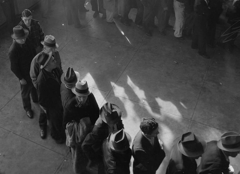
Line of men in San Francisco, California, waiting to register for unemployment benefits in January 1938, on one of the first days they were made available in that state.
Employment rent
We can now determine Bob’s employment rent if he had kept his original job at the steel mill for six months. We will assume the six-month period starts at the beginning of January and goes until the end of June. Figure 11.3 models his employment rent over this period.

Figure 11.3 The size of Bob’s employment rent for six months in his original job compared to losing that job and getting income from unemployment insurance.
If Bob keeps his job at the steel mill and his alternative is to lose his job and get the fallback option of six months of unemployment insurance, then his employment rent is his total earnings from his job at the steel mill for six months, minus the income from his fallback (the monthly unemployment insurance) and the personal cost of working at the steel mill. The remaining value is his employment rent or his cost of losing the job.

Bob’s earnings from his job at the steel mill for six months if he is not fired

Bob’s income from six months of unemployment insurance

Bob’s personal cost of working at the steel mill for six months

Subtracting out cost of work and outside option

Bob’s employment rent
As in Figure 11.2, the red line represents Bob’s path if he loses his job and then is hired at an equivalent job with the same pay after six months. The blue line represents his path if he keeps his current job over those six months. The red area at the bottom represents the total income he will receive from six months of unemployment benefits (his fallback option). Stacked above that, the green area is Bob’s personal cost of working. The blue area is his employment rent, which is what he will lose if he loses his job.
Any change in the costs and benefits of a worker’s current job and outside option will affect the employment rent. This has some important implications.
First, employers have some control over their workers’ employment rents. If an employer wants to increase the employment rents for its workers, they could:
- raise wages
- reduce the personal cost of working by improving working conditions.
This video from Vox explains some of the difficulties in the way unemployment benefits are distributed in the United States. It shows how states differ in their levels of benefits, restrictions on who can get them, and ease of access. These differences affect employment rents.
Second, governments can affect the size of employment rents by changing the rules of the game. Unemployment benefits are an especially important example. Governments set the size and duration of unemployment benefits. A change in either affects employment rents for many workers.

Job seekers line up to get a job at a Jamba Juice. As unemployment increases, open positions will attract more applicants, resulting in longer periods of unemployment for those without a job.
Third, employment rents are affected by the economy’s unemployment rate. Imagine that when Bob started his job, the unemployment rate was 3.5%. But by the beginning of the following year, the unemployment rate was 6%. Higher unemployment means there will be more competition among workers for fewer open jobs.
So, if Bob loses his job, he expects to be unemployed longer than he would have been when the unemployment rate was lower. He may even have to extend his unemployment benefits over a longer period, which will decrease his monthly spending. He may also expect that any job he can find will pay less than it paid when the unemployment rate was lower. Both of these changes decrease the net benefit of his outside option and so raise his employment rent. Extension 11.4 describes how we can model the effect of higher unemployment on Bob’s employment rent.
Why employment rents give employers power
Employers benefit from employment rents in two critical ways:
- The worker is more likely to stay with the firm. The bigger a worker’s employment rent, the more likely they are to remain at the job. The employer therefore does not have to hire and train a new worker.
- The employer can threaten to fire the worker. A larger employment rent means a larger cost to the worker of losing their job, which in turn makes the threat of being fired more effective and makes workers act in ways they would not likely do otherwise. A larger employment rent, in other words, increases the bargaining power of employers.
- structural power
- The extent of a person or firm’s advantage in a bargain that is determined by the relative value of their next-best alternative to the bargain.
Labor unions, in addition to improving the bargaining power of workers, can affect the structural power of employers by pressuring governments to improve the outside option of workers. In Chapter 2, for example, we learned how unions helped pass the Fair Labor Standards Act (FLSA) of 1938. The FLSA, by implementing a federal minimum wage, introducing overtime pay, and prohibiting child labor, improved the outside option for many workers.
A worker’s outside option affects the size of their employment rent at a given wage, and outside options are therefore connected to an employer’s structural power. Any change that increases the net benefit of a worker’s outside option decreases employers’ structural power.
Everyday Economics 11.7
During the COVID-19 pandemic, the federal government increased unemployment benefits by $600 per week (reduced to $300 per week later) and extended the eligibility period for unemployment benefits from 26 weeks before the pandemic to 53 weeks during the pandemic. How did this policy change affect employment rents for workers? How did it affect employers’ structural power? How do you think many low-wage workers responded to this change? How do you think employers responded?
For example, as the unemployment rate goes up, the outside option for workers gets worse, increasing the employer’s structural power. A weaker outside option makes it harder for workers to quit or turn down a job offer, and the wage that employers need to offer to incentivize workers to work will decrease.
In the next section, we apply what we’ve learned so far in this chapter to better understand some of the questions we raised in Section 11.1, such as how wages and effort levels are determined.
Extension 11.4 How higher unemployment affects the employment rent
The blue line is the same, however, because the increase in unemployment does not affect the costs or benefits of Bob’s current job. His outside option is worse and his current job is equally valuable, and so his employment rent increases, which you can see because the gap between the blue and red lines is bigger in Figure E11.2 than in Figure 11.3.

How an increase in the unemployment rate affects the employment rent
Figure E11.2 How an increase in the unemployment rate affects the employment rent When the unemployment rate increases, workers expect to be unemployed for longer than normal. In this case, Bob expects to be unemployed for nine months rather than six months. But his unemployment benefits last for only six months. He now has to spread his unemployment benefits across nine months. His fallback is therefore worth less per month than if his period of unemployment is only six months. With the same personal cost of work per month, his employment rent if he keeps his job is therefore larger when the unemployment rate is higher. Thus, Bob’s cost of losing his job is greater when the unemployment rate is higher—he knows it’s harder to get a job, and so it’s worse for him to lose his job compared to when the unemployment rate is lower.

Bob’s earnings from his job at the steel mill for nine months if he is not fired

Bob’s income from six months of unemployment insurance spread across nine months

Bob’s personal cost of working for nine months
Bob’s employment rent is larger with higher unemployment
Lower unemployment, on the other hand, will increase the value of his outside option, lowering his employment rent. An example of this scenario is the difference in lost earnings for those who lost their job during a recession compared to those who lost their job in an expansion, which we saw in Figure 11.1.
Exercise E11.5 How slowing job creation affects firms, workers, and hiring platforms
Read this article about hiring sites such as LinkedIn and Indeed that are affected by slowing job creation and rising unemployment. Then answer the following questions.
- Why do hiring sites lose revenue during periods of slowing job creation and rising unemployment? How are they responding to these challenges?
- If a firm is hiring during such a period, what are the advantages to the firm? What are the disadvantages to the firm?
- The article contains comments from Boston University marketing professor Andrey Fradkin. Based on his comments, how do job hiring sites affect a worker’s outside option and employment rent?
- Based on what you read in the article, do you expect unemployed workers to have increased or decreased wages at a new job compared to an old job? How are the employment rents of workers who keep their jobs affected?
Question E11.5
How does an increase in the unemployment rate affect a worker’s outside option? Choose all that apply.
- Higher unemployment increases competition among workers, not firms, so outside options do not improve.
- A higher unemployment rate makes job search longer and more difficult, reducing the value of the outside option.
- The outside option is sensitive to labor market conditions, so it changes.
- When benefits must be stretched over a longer time, monthly support falls, weakening the outside option.
Exercise 11.6 How does falling unemployment affect workers?
Explain how and why a decrease in the unemployment rate will affect each of the following for Bob, assuming he keeps his current job.
- Net benefit of keeping his job
- Net benefit of outside option
- Employment rent
- Bob’s structural power
Exercise 11.7 Employer-sponsored health insurance and employment rents
In 2023, about 60% of people under the age of 65 had employer-sponsored health insurance (ESI), meaning that their health insurance was purchased either through their employer or the employer of a family member.
- How does having ESI affect a worker’s employment rents?
- Imagine that the rules of the game change in the United States such that ESIs are no longer an option and everyone is provided with good health insurance that they will always have, regardless of their job or employment status. However, this change comes with higher taxes, meaning that average disposable income decreases. How will this change in our institutions affect the quality of matches in the labor market? How will it affect employment rents?
- ESI is uncommon in the rest of the world. Pick a few other countries and research how their health insurance system works. Describe your findings. How do you think these different systems affect employment rents and quality of matches in the labor market?
Question 11.5
At a manufacturing plant, AutoBuild, workers are becoming more anxious than before about potential layoffs. They now believe that finding another job in their industry could take several months, whereas before they expected they could find another job in a few weeks. How does this higher level of anxiety affect the employment rent of AutoBuild’s workers?
- If it now takes longer to find another job, the outside option worsens, so the cost of losing the current job is higher and employment rent increases.
- Because the outside option has changed, employment rent cannot stay the same.
- A weaker outside option makes the job more valuable, so employment rent rises, not falls.
- The effect is clear: Employment rent goes up when it is harder to find another job.
Question 11.6
In which of the following situations will the employment rent be relatively high, ceteris paribus? Choose all that apply.
- If the employee loses the job, all these benefits will be lost, and so the economic rent from employment is high.
- The cost of job loss is low, because it will be easy to find another job. Therefore, the economic rent is low.
- A qualified accountant will be able to find other jobs easily at a similar salary, so the economic rent is low.
- This worker is paid a high salary because of firm-specific assets that will be lost if they leave. Other firms will pay a lower salary (at least initially), so the economic rent is high.
