4.5 Production functions: Turning inputs into outputs

So far, we’ve modeled how firms choose a technology for producing a given amount of output, but firms also vary the amount of output they produce.

In this section, we examine how technology and technological progress affect the relationship between input and output, deepening our understanding of why technological progress is instrumental in lifting people out of poverty. We model a simple example of a farmer, Angela, who produces grain on a farm that she owns and works.

Angela’s technology: Producing grain with hours of work

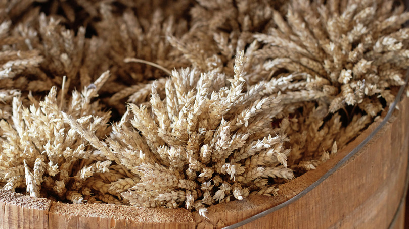
Mature ears of grain wheat.

The amount of grain Angela can produce depends on the technology she uses and how many hours she works each day. Like the old Midwestern farmers described in Section 4.1, Angela’s technology involves the use of hand tools, horses, and mules. Table 4.3 shows how the amount of grain produced depends on how many hours Angela works. For example, by working for five hours, Angela can produce 37.3 bushels of grain.

What’s a bushel of grain? A bushel is a unit of volume. It is also the name of a container (a bushel basket), and the capacity of the container becomes a bushel of the grain stored. In 1866, a grain wheat farmer in the United States harvested, on average, 11.0 bushels per acre per year. In 2019, that number was 51.7 bushels per acre per year. Angela’s harvest is therefore consistent with modern numbers of how many bushels per acre per year a farmer will harvest depending on varying weather and other conditions.

production function

A production function is a graphical or mathematical description of the relationship between the quantities of the inputs to a production process and the amount of output produced.

Table 4.3 represents a production function, which is the relationship between the inputs to a production process—such as the hours of work a farmer like Angela puts in—and the amount of output, such as the bushels of grain. In this example, there are two inputs: labor and land. Because the amount of land Angela works on is a fixed amount, Table 4.3 includes only the labor input, Angela’s hours of work.

Following the principle of trade-offs and opportunity costs, Angela must give up free time to harvest more grain. As she works more, however, she harvests less grain for each additional hour she works. As Table 4.3 shows, she gets more grain from the first hour of work than the second, more from the second than the third, and so on. She gets these results because the amount of land available is fixed: Working twice as many hours on the same amount of land will not double its output.

marginal product of labor

The marginal product of an input to production (for example, the marginal product of labor) is the additional amount of output produced in response to a 1-unit increase in the input.

To understand Angela’s production decision, we need to look at the average product of labor and the marginal product of labor. Both numbers are shown in Table 4.3. The marginal product of labor is the additional grain Angela produces from one extra hour of work. For example, if Angela increases her hours of work from two hours with a total output of 24 bushels to three hours with a total output of 29 bushels, then she produces an extra five bushels from the additional hour of work. The marginal product of her third hour of work is five bushels.

The average product and the marginal product of labor decrease as Angela’s number of hours worked increases. This technology therefore has a diminishing average product of labor. Past a certain point, spending another hour out in the fields will not be worth the effort. When that happens, improving her standard of living will require technological progress.

Technological progress and the production function

We can use the data in Table 4.3 to draw a smoothed-out graph of the production function, which helps us visualize how technological progress affects Angela’s standard of living. Figure 4.7 plots the number of hours worked on the horizontal axis, and the corresponding output of grain on the vertical axis.

Fullscreen

https://books.core-econ.org/uoe-101/04-05.html#figure-4-7

Figure 4.7 Angela’s production function of grain (the output) with hours of work time (the input) using a given production technology. The difference between points T and R shows Angela’s decreasing marginal product and decreasing average product of labor.

Fullscreen

https://books.core-econ.org/uoe-101/04-05.html#figure-4-7a

Hours of work and bushels of grain on the axes

To understand how Angela produces grain, we can plot her hours of work on the horizontal axis and the number of bushels of grain she produces on the vertical axis.

Fullscreen

https://books.core-econ.org/uoe-101/04-05.html#figure-4-7b

Plotting the points

Using Table 4.3, we plot each combination of labor and output, with one dot for each value of Angela’s hours of work time on the horizontal axis and the corresponding amount of grain (in bushels) on the vertical axis.

Fullscreen

https://books.core-econ.org/uoe-101/04-05.html#figure-4-7c

Drawing the production function

The production function for turning hours of work into bushels of grain shows how each value of Angela’s hours of work time produces a corresponding amount of grain. The production function is shown in red. Despite not having all the points between each hour of work, we simplify by drawing a smooth line between them.

Fullscreen

https://books.core-econ.org/uoe-101/04-05.html#figure-4-7d

Reading a point on the production function

When Angela works five hours, she produces 37.3 bushels of grain, as shown at point T. She also has 19 hours of free time. The arrows show her work time compared to her free time.

Fullscreen

https://books.core-econ.org/uoe-101/04-05.html#figure-4-7e

Angela’s output when working six hours

When Angela works six hours, she produces 40.6 bushels of grain, as shown at point R. She also has 18 hours of free time. The arrows show her work time compared to her free time.

Fullscreen

https://books.core-econ.org/uoe-101/04-05.html#figure-4-7f

Calculating the marginal product

Comparing points T and R, we see that the difference in the amount of Angela’s production is Angela’s marginal product of her 6th hour of work: 40.6 – 37.3 = 3.3 bushels of grain, which is the marginal product of going from five hours of work to six hours of work (a difference of 1 hour).

In Figure 4.7, the production function slopes upward, reflecting the fact that Angela can harvest more grain as she works more hours. The shape of the production function also captures the decreasing average product of labor, because it starts to flatten out and increase more slowly as the hours increase.

Now suppose Angela buys a tractor to replace her horses and mules. The tractor will allow her to produce more grain per hour than before. Figure 4.8 shows how this technological progress affects her production function. The starting point will remain the same because regardless of her technology, zero hours of work will produce zero output. But for any number of hours worked, she can produce more than before. Technological progress results in the curve rotating upwards.

Fullscreen

https://books.core-econ.org/uoe-101/04-05.html#figure-4-8

Figure 4.8 Angela’s original production function (red) and new production function with new farming tools (blue).

Fullscreen

https://books.core-econ.org/uoe-101/04-05.html#figure-4-8a

Working six hours with horses and mules

This is Angela’s original production function, prior to her purchase of a tractor. We will assume that she works six hours a day, producing 40.6 bushels of grain.

Fullscreen

https://books.core-econ.org/uoe-101/04-05.html#figure-4-8b

Angela’s production function with a tractor

After buying a tractor, Angela’s production function rotates upwards. The starting point will remain the same because zero hours of work will still produce zero output. But because a tractor is more productive than horses and mules, she can produce more for any number of hours worked.

Fullscreen

https://books.core-econ.org/uoe-101/04-05.html#figure-4-8c

Angela can produce more grain with six hours of work

If Angela continues to work six hours per day with the new technology, she will move from point R to point S. She will now be harvesting 50.7 bushels a day instead of 40.6.

Fullscreen

https://books.core-econ.org/uoe-101/04-05.html#figure-4-8d

Angela can produce the same amount as before with less work

If Angela is happy producing 40.6 bushels per day, she can continue to produce that amount. With the new technology, she can produce that output in 3.75 hours instead of six hours. In this case, she will move from point R to point Q.

Suppose Angela originally worked six hours per day, producing 40.6 bushels of grain (point R). With the new technology, she can produce 50.7 bushels a day without changing her hours of work (point S). Or, if she’s happy producing 40.6 bushels per day, she can now produce that amount in 3.75 hours (point Q). Regardless of how many hours she will work producing grain, the adoption of the tractor gives her more options and the ability to increase her standard of living, as she can increase both her free time and her grain production. Additional technological progress, such as an even better tractor, will further expand her options and further increase her standard of living.

In this section from The Economy: A South Asian Perspective, you can see the technological progress that has been made in wheat production in the United States.

Gross Domestic Product (GDP)

A measure of the total output of goods and services produced in an economy in a given period. GDP combines in a single number all the output (or production) carried out by the firms, nonprofit institutions, and government bodies within a country. Household production is part of GDP if it is sold.

The example helps us understand why technological progress is critical to the increasing GDP per capita we saw in Chapter 3. Aside from working longer hours, the only way society can produce more is to reduce the resources needed to produce the things we already make. Without ongoing technological progress in food production freeing up resources and workers, we would still be spending much of our time producing food.

So far, we have focused mainly on the technological decisions and production outcomes for individual firms. In the next section, we describe how specialization can improve average living standards.

Math Extension 4.5 Decreasing, constant, and increasing returns to scale

decreasing returns to scale

When production exhibits decreasing returns to scale, increasing all of the inputs to a production process by the same proportion increases output by a lower proportion.

A production function with a diminishing average product of labor, like those in Figures 4.7 and 4.8, is not unusual for many agricultural products. Most agricultural production is characterized by decreasing returns to scale, which occurs when the marginal product decreases as the input increases. For example, with decreasing returns to scale, increasing input by 10% will cause output to increase by less than 10%. Decreasing returns to scale are common for agricultural products because increasing input typically entails expanding to land not as well-suited to that crop.

constant returns to scale

When production exhibits constant returns to scale, increasing all of the inputs to a production process by the same proportion increases output by the same proportion.

Now let’s look at another example. Consider what the production function for a call center might be. For the sake of simplicity, assume that workers are the only input, and each worker works an eight-hour shift. Also assume that each worker is able to handle 50 calls per shift. In this case, adding one more unit of input (one worker) will result in 50 more units of output (calls handled), which means that the marginal product is always the same. This phenomenon is called constant returns to scale.

A production function with constant returns to scale has a different shape than one with decreasing returns to scale. Figure E4.5 shows a production function for our imagined call center. Unlike Figures 4.7 and 4.8, which are curved, this function is linear, which is why it graphs as a straight line. From any point, increasing the input by X% increases the output by X%. For example, imagine you start with 10 workers handling 500 calls. Increasing the input (the number of workers) by 20% means you now have (10 × 1.2) = 12 workers. Similarly, the output will increase by 20%, which in this case is (500 × 1.2) = 600.

Fullscreen

https://books.core-econ.org/uoe-101/04-05.html#figure-e4-5

Figure E4.5 A production function with constant returns to scale.

increasing returns to scale

No definition available.

economies of scale

When production exhibits increasing returns to scale, increasing all of the inputs to a production process by the same proportion increases the output by a higher proportion.

A production function can also have increasing returns to scale (often called economies of scale), which occurs when the marginal product increases as the input increases. For example, with increasing returns to scale, increasing input by 10% will increase output by more than 10%. Economies of scale are common in capital-intensive industries.

Figure E4.6 shows what a production function with economies of scale might look like. Because the marginal product increases as your input increases, the curve gets steeper as you go from left to right.

Fullscreen

https://books.core-econ.org/uoe-101/04-05.html#figure-e4-6

Figure E4.6 A production function with increasing returns to scale.

These three types of production function can also be combined. You may have a technology that, depending on the level of input, has increasing returns, decreasing returns, or constant returns to scale. The outcome will depend on the complicated relationships between capital, workers, and inputs that often exist in modern production.

Question E4.3

Which of the following statements about constant returns to scale are correct? Choose the correct option(s).

• Doubling all inputs results in exactly double the output.
• Output increases in the same proportion as input increases.
• Output increases more than proportionally with input.
• Agricultural production typically exhibits constant returns to scale.

• This is the definition of constant returns to scale.
• This is another way of stating that output scales 1:1 with inputs.
• This describes increasing returns to scale.
• Agricultural production often shows decreasing returns to scale, not constant returns to scale.

Exercise E4.3 Production function and returns to scale

What type of returns to scale does this production function exhibit? Show your reasoning.

Workers	Output
4	100
8	240
12	420